Single CDR3 amino acid swaps

Look at pairs of CMV ECOcluster TCRs that differ by one amino acid swap. They’re strongly position-dependent!

1 Takeaways from this post

• There are >50,000 pairs of CMV ECOcluster TCRs that differ by a single amino acid substitution in the CDR3 sequence
  • A priori, I expect those pairs overwhelmingly to represent TCRs binding the same CMV antigen presented by the same HLA allele
  • They behave like they do
• Amino acid swaps are strongly concentrated in a single CDR3 position relative to the V gene
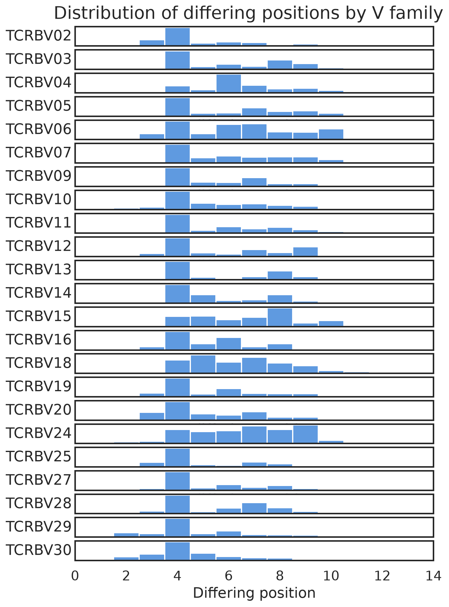
  • The specific position varies strongly by V family
  • For most V families, it’s position 4 (0-based)
  • Interpretation: AA swaps immediately after the V gene end are more tolerated in TCR-pMHC binding solutions
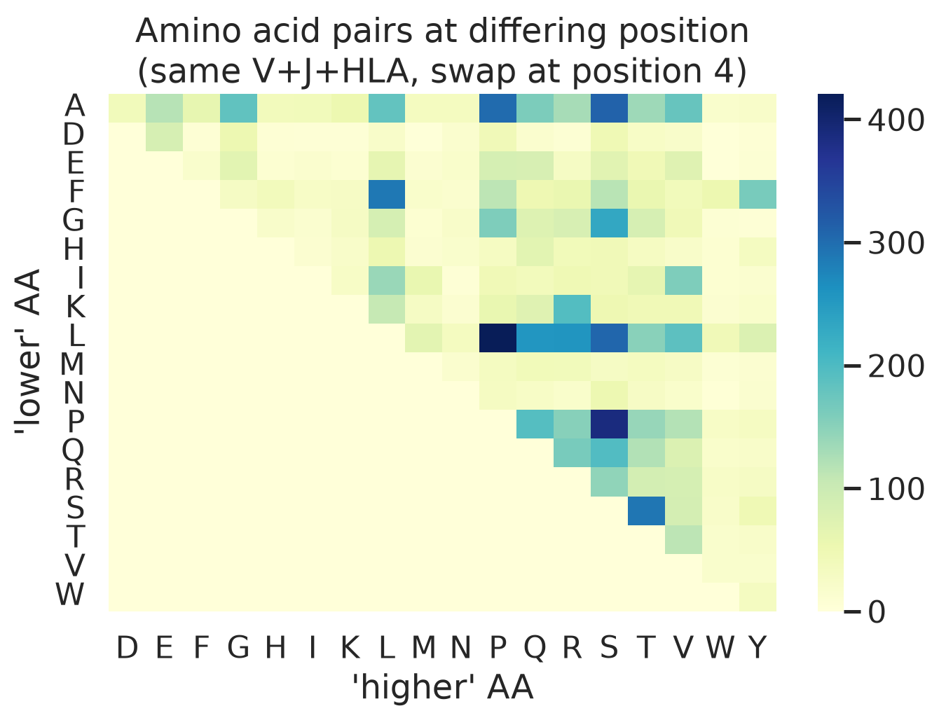
• Some amino acid pairs are swapped far more or less often than we’d expect by chance
  • We could use this data to build a BLOSUM-like matrix for CDR3 sequences with respect to pMHC binding
• Both those kinds of restrictions could be used to inform distance metrics and clustering algorithms on TCRs

2 Background

In Post 4, I looked at the 2026 CMV ECOcluster and found that many CDR3 sequences are present in multiple TCRs, with different V and/or J genes. In this post, I look at pairs of TCRs that differ by a single amino acid substitution in the CDR3 sequence. I’m curious what kinds of amino acid swaps (in terms of position in sequence and AA identity) are best tolerated.

I’m making a big assumption here: in this rarified context in which I know that all these TCRs are CMV-specific, a pair of TCRs with the same CDR3 length and a single amino acid substitution binds the same antigen.

That is, I don’t know how to perfectly cluster TCRs to identify groups that bind the same antigen in the general case (and I’d argue that no one does), but in this context in which both TCRs are CMV ECOcluster members I think this “smallest possible”* change to a CDR3 doesn’t affect which CMV pMHC complex the TCR binds. I’ll explore that assumption a little bit here, and more in a later post where I look at public TCR databases.

* All single AA swaps aren’t actually the smallest possible changes to a CDR3. Not all single AA swaps are created equal, as we’ll see.

3 Load the 2026 CMV ECOcluster and find Hamming-1 CDR3 pairs

I’m finding all pairs of CMV ECOcluster TCRs with the same CDR3 length that differ by one amino acid in one position. I’m not considering whether the V and J genes are the same or not, or whether the two TCRs are associated with the same HLA allele.

I’m doing it that way so that I can see what kinds of “confusion” there seems to be between pairs of V genes, J genes and HLA associations.

# useful imports
import pandas as pd
from matplotlib import pyplot as plt

import itables
import seaborn as sns
from cmvividly.plots.style import set_style
set_style()

import itables
itables.init_notebook_mode()

#stats
from scipy.stats import mannwhitneyu

from cmvividly.data.access import load_cmv_ecocluster_2026, load_cmv_ecocluster_2026_cdr3_hamming1_pairs
from cmvividly.data.hamming1_pairs import populate_hamming1_pairs_othercols

pdf_cmv_ecocluster_2026 = load_cmv_ecocluster_2026()
pdf_all_ham1_pair_rows = load_cmv_ecocluster_2026_cdr3_hamming1_pairs()

# add a bunch of useful columns to the Hamming-1 pairs dataframe
pdf_all_ham1_pairs = populate_hamming1_pairs_othercols(pdf_all_ham1_pair_rows, pdf_cmv_ecocluster_2026)
pdf_all_ham1_pairs["same_vj"] = pdf_all_ham1_pairs.same_vgene & pdf_all_ham1_pairs.same_jgene
pdf_all_ham1_pairs["vgene_lower"] = pdf_all_ham1_pairs[["vgene_i", "vgene_j"]].min(axis=1)
pdf_all_ham1_pairs["vgene_higher"] = pdf_all_ham1_pairs[["vgene_i", "vgene_j"]].max(axis=1)
# add a column indicating which position in the CDR3 sequence is swapped, counting from the J end
pdf_all_ham1_pairs["differing_position_fromj"] = pdf_all_ham1_pairs["cdr3_j"].str.len() - pdf_all_ham1_pairs["differing_position"]
# add columns describing the AA swap
pdf_all_ham1_pairs["aa_i"] = [
    row["cdr3_i"][row["differing_position"]] for _, row in pdf_all_ham1_pairs.iterrows()]
pdf_all_ham1_pairs["aa_j"] = [
    row["cdr3_j"][row["differing_position"]] for _, row in pdf_all_ham1_pairs.iterrows()]
pdf_all_ham1_pairs["aa_lower"] = pdf_all_ham1_pairs[["aa_i", "aa_j"]].min(axis=1)
pdf_all_ham1_pairs["aa_higher"] = pdf_all_ham1_pairs[["aa_i", "aa_j"]].max(axis=1)
pdf_all_ham1_pairs["aa_pair"] = pdf_all_ham1_pairs["aa_lower"] + pdf_all_ham1_pairs["aa_higher"]
pdf_all_ham1_pairs["cdr3_len"] = pdf_all_ham1_pairs["cdr3_i"].str.len()
pdf_ham1_pairs_samehla_samevj = pdf_all_ham1_pairs[
    (pdf_all_ham1_pairs.same_vj) & (pdf_all_ham1_pairs.same_hla)]

tcrs_in_pairs = set(pdf_all_ham1_pairs.tcr_i)
tcrs_in_pairs.update(set(pdf_all_ham1_pairs.tcr_j))
print(f"Loaded {len(pdf_all_ham1_pairs):,} CDR3 Hamming-1 pairs (on {len(tcrs_in_pairs):,} total TCRs) from the {len(pdf_cmv_ecocluster_2026):,}-TCR 2026 CMV ECOcluster.")
pdf_all_ham1_pairs[["cdr3_i", "cdr3_j", "differing_position", "aa_pair", "same_vgene", "same_jgene", "same_hla", "vgene_i", "vgene_j", "jgene_i", "jgene_j", "hla_i", "hla_j"]]

Loaded 55,622 CDR3 Hamming-1 pairs (on 31,742 total TCRs) from the 52,447-TCR 2026 CMV ECOcluster.

ⓘcdr3_i	cdr3_j	differing_position	aa_pair	same_vgene	same_jgene	same_hla	vgene_i	vgene_j	jgene_i	jgene_j	hla_i	hla_j
CASSLSGTGGWNEQFF	CASSLSGTGGLNEQFF	10	LW	False	True	False	TCRBV07-02	TCRBV05-06	TCRBJ02-01	TCRBJ02-01	DRB1*07:01	DRB1*01:01
CASSHFGTGGNTEAFF	CASSQFGTGGNTEAFF	4	HQ	True	True	True	TCRBV05-06	TCRBV05-06	TCRBJ01-01	TCRBJ01-01	DRB1*07:01	DRB1*07:01
CASSHFGTGGNTEAFF	CASSLFGTGGNTEAFF	4	HL	True	True	True	TCRBV05-06	TCRBV05-06	TCRBJ01-01	TCRBJ01-01	DRB1*07:01	DRB1*07:01
CASSHFGTGGNTEAFF	CASSFFGTGGNTEAFF	4	FH	True	True	True	TCRBV05-06	TCRBV05-06	TCRBJ01-01	TCRBJ01-01	DRB1*07:01	DRB1*07:01
CASSHFGTGGNTEAFF	CASSSFGTGGNTEAFF	4	HS	True	True	True	TCRBV05-06	TCRBV05-06	TCRBJ01-01	TCRBJ01-01	DRB1*07:01	DRB1*07:01
CASSQFGTGGNTEAFF	CASSLFGTGGNTEAFF	4	LQ	True	True	True	TCRBV05-06	TCRBV05-06	TCRBJ01-01	TCRBJ01-01	DRB1*07:01	DRB1*07:01
CASSQFGTGGNTEAFF	CASSFFGTGGNTEAFF	4	FQ	True	True	True	TCRBV05-06	TCRBV05-06	TCRBJ01-01	TCRBJ01-01	DRB1*07:01	DRB1*07:01
CASSQFGTGGNTEAFF	CASSSFGTGGNTEAFF	4	QS	True	True	True	TCRBV05-06	TCRBV05-06	TCRBJ01-01	TCRBJ01-01	DRB1*07:01	DRB1*07:01
CASSLFGTGGNTEAFF	CASSFFGTGGNTEAFF	4	FL	True	True	True	TCRBV05-06	TCRBV05-06	TCRBJ01-01	TCRBJ01-01	DRB1*07:01	DRB1*07:01
CASSLFGTGGNTEAFF	CASSSFGTGGNTEAFF	4	LS	True	True	True	TCRBV05-06	TCRBV05-06	TCRBJ01-01	TCRBJ01-01	DRB1*07:01	DRB1*07:01
(55,612 more rows not shown)

4 Break down Hamming-1 pairs by same or different V/J gene and HLA allele

In Post 4, I looked at full CDR3s present in multiple TCRs (necessarily with different V or J gene) and observed some trends. Do the trends here look the same?

In how many of these pairs do both TCRs have the same V gene, same J gene, both or neither?

display(pd.crosstab(pdf_all_ham1_pairs.same_vgene, pdf_all_ham1_pairs.same_jgene))

ⓘsame_jgene	False	True
same_vgene
False	227	15194
True	1261	38940

pdf_all_ham1_pairs[~pdf_all_ham1_pairs.same_vgene][["vgene_lower", "vgene_higher"]].value_counts().reset_index()

ⓘvgene_lower	vgene_higher	count
TCRBV20-01	TCRBV20-X	1266
TCRBV07-02	TCRBV07-03	392
TCRBV06-05	TCRBV06-X	298
TCRBV07-06	TCRBV07-X	282
TCRBV05-01	TCRBV06-05	263
TCRBV07-02	TCRBV07-X	223
TCRBV06-05	TCRBV06-06	219
TCRBV07-02	TCRBV19-01	182
TCRBV07-02	TCRBV07-08	171
TCRBV07-02	TCRBV07-07	167
(817 more rows not shown)

Looks like there’s a lot more V gene confusion than J gene, and the confused V genes are consistent with what I found in Post 4. And it’s the same story on the J gene side (not shown).

How many of these pairs have both TCRs associated with the same HLA allele?

display(pdf_all_ham1_pairs.same_hla.value_counts().reset_index())

ⓘsame_hla	count
True	40340
False	15282

pdf_all_ham1_pairs_diff_hla = pdf_all_ham1_pairs[~pdf_all_ham1_pairs.same_hla]
# make a new column, hla_lower, with the lexicographically lower of hla_i and hla_j
pdf_all_ham1_pairs_diff_hla["hla_lower"] = pdf_all_ham1_pairs_diff_hla[["hla_i", "hla_j"]].min(axis=1)
pdf_all_ham1_pairs_diff_hla["hla_higher"] = pdf_all_ham1_pairs_diff_hla[["hla_i", "hla_j"]].max(axis=1)
pdf_all_ham1_pairs_diff_hla[["hla_lower", "hla_higher"]].value_counts().reset_index()

ⓘhla_lower	hla_higher	count
DQA1*01:02+DQB1*06:02	DRB5*01:01	1288
DRB1*15:01	DRB5*01:01	1099
DQA1*01:01+DQB1*05:01	DQA1*01:05+DQB1*05:01	1006
DQA1*01:03+DQB1*06:03	DRB1*13:01	786
DQA1*01:01+DQB1*05:01	DRB1*01:01	407
DPA1*01:03+DPB1*03:01	DPA1*01:03+DPB1*104:01	380
DQA1*01:02+DQB1*06:02	DRB1*15:01	372
DQA1*01:05+DQB1*05:01	DRB1*01:01	347
DQA1*05:01+DQB1*02:01	DRB1*03:01	234
DQA1*05:05+DQB1*03:01	DRB1*11:01	230
(1,456 more rows not shown)

Again, similar story to the pairs of TCRs with the same CDR3: when there’s confusion, it’s concentrated in a few pairs of HLA alleles. Likely, they’re alleles the HLA models can’t distinguish very well because of LD or similar TCR binding.

The 1-Hamming CDR3 pairs are behaving much like the identical CDR3 pairs, consistent with the idea that these single amino acid swaps, in which both TCRs are CMV ECOcluster members, don’t change which pMHC the TCR binds.

5 Where in the CDR3 sequence do these substitutions occur?

For starters, I’ll define the “position” of the amino acid substution as a zero-based index starting from the N terminus (V gene end). So, e.g.:

C A S S H F G T G G N T E A F F

0 1 2 3 4 5 6 7 8 9 10 11 12 13 14 15

Let’s look at the distribution of substitutions by position in the CDR3 sequence. Naturally, we might expect that distribution to differ by CDR3 length.

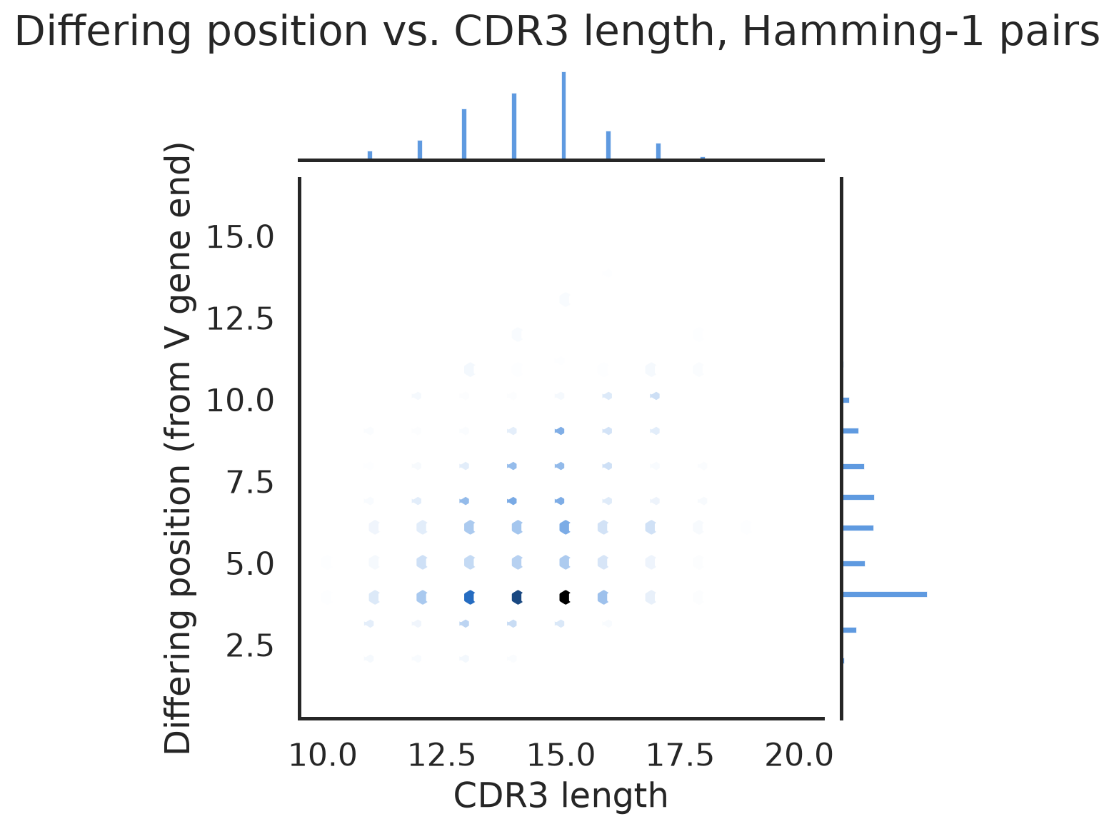
G = sns.jointplot(data=pdf_all_ham1_pairs,
            x="cdr3_len", y="differing_position", kind="hex")
G.set_axis_labels("CDR3 length", "Differing position (from V gene end)")
G.fig.suptitle("Differing position vs. CDR3 length, Hamming-1 pairs", y=1.02)
pass

Well, that’s strange! Position 4 (the fifth amino acid, as in the H in CASSHFGTGGNTEAFF) is by far the most commonly substituted position. And that seems to be the case regardless of CDR3 length.

What proportion of total Hamming-1 pairs does position 4 represent?

proportion_pos4 = sum(pdf_all_ham1_pairs.differing_position == 4) / len(pdf_all_ham1_pairs)
print(f"Proportion of Hamming-1 pairs differing at position 4: {proportion_pos4:.2%}")

Proportion of Hamming-1 pairs differing at position 4: 34.95%

I could do some statistics around that, but there’s no point: that’s far more than expected by chance.

Let’s try to eliminate the possibility that this is some kind of artifact.

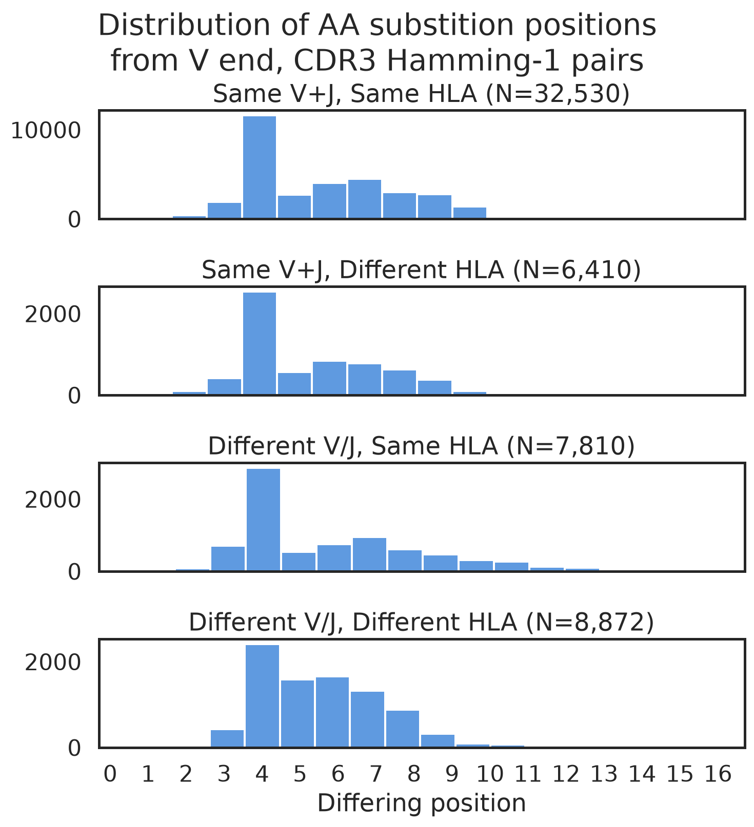
Let’s look at the distribution of differing positions for all Hamming-1 pairs, broken down by whether the two TCRs have the same V and J genes, and whether they have the same HLA allele association. Maybe this only happens when the two TCRs have different V/J genes or allele associations.

def hist_differing_positions(pdf_all_ham1_pairs, position_col, v_or_j_side):
    f, (ax1, ax2, ax3, ax4) = plt.subplots(4, 1, figsize=(8, 8), sharex=True)
    pdf_samevj_samehla = pdf_all_ham1_pairs[pdf_all_ham1_pairs.same_vj & pdf_all_ham1_pairs.same_hla]
    pdf_samevj_diffhla = pdf_all_ham1_pairs[pdf_all_ham1_pairs.same_vj & ~pdf_all_ham1_pairs.same_hla]
    pdf_diffvj_samehla = pdf_all_ham1_pairs[~pdf_all_ham1_pairs.same_vj & pdf_all_ham1_pairs.same_hla]
    pdf_diffvj_diffhla = pdf_all_ham1_pairs[~pdf_all_ham1_pairs.same_vj & ~pdf_all_ham1_pairs.same_hla]

    sns.histplot(x=position_col, hue="same_hla",
                  data=pdf_samevj_samehla, multiple="dodge", bins=pdf_samevj_samehla[position_col].max() - pdf_samevj_samehla[position_col].min() + 1,
                 common_norm=False, ax=ax1)
    ax1.set_title(f"Same V+J, Same HLA (N={len(pdf_samevj_samehla):,})")
    sns.histplot(x=position_col, hue="same_hla",
                  data=pdf_samevj_diffhla, multiple="dodge", bins=pdf_samevj_diffhla[position_col].max() - pdf_samevj_diffhla[position_col].min() + 1,
                 common_norm=False, ax=ax2)
    ax2.set_title(f"Same V+J, Different HLA (N={len(pdf_samevj_diffhla):,})")
    sns.histplot(x=position_col, hue="same_hla",
                  data=pdf_diffvj_samehla, multiple="dodge", bins=pdf_diffvj_samehla[position_col].max() - pdf_diffvj_samehla[position_col].min() + 1,
                 common_norm=False, ax=ax3)
    ax3.set_title(f"Different V/J, Same HLA (N={len(pdf_diffvj_samehla):,})")
    sns.histplot(x=position_col, hue="same_hla",
                  data=pdf_diffvj_diffhla, multiple="dodge", bins=pdf_diffvj_diffhla[position_col].max() - pdf_diffvj_diffhla[position_col].min() + 1,
                 common_norm=False, ax=ax4)
    ax4.set_title(f"Different V/J, Different HLA (N={len(pdf_diffvj_diffhla):,})")
    # force all xticks for ax4, the one we'll be labeling
    ax4.set_xticks([x + 0.3 for x in range(0, max(pdf_all_ham1_pairs[position_col]) + 1)])
    ax4.set_xticklabels([str(x) for x in range(0, max(pdf_all_ham1_pairs[position_col]) + 1)])
    for ax in [ax1, ax2, ax3, ax4]:
        ax.get_legend().remove()
        ax.set_ylabel("")
        ax.set_xlim(0, max(pdf_all_ham1_pairs[position_col]) + 1)
    #for ax in [ax1, ax2, ax3]:
    #    ax.set_xticks([])
    ax4.set_xlabel("Differing position")
    f.tight_layout()
    f.suptitle(f"Distribution of AA substition positions\nfrom {v_or_j_side} end, CDR3 Hamming-1 pairs", y=1.06)

hist_differing_positions(pdf_all_ham1_pairs, "differing_position", "V")

It doesn’t matter whether we’re talking about TCR pairs with the same V and J genes, or the same HLA allele assocations, or not. No matter how you slice it, Position 4 is an outlier.

On the face of it, that suggests that mutations affecting position 4 are more tolerated than mutations affecting other positions.

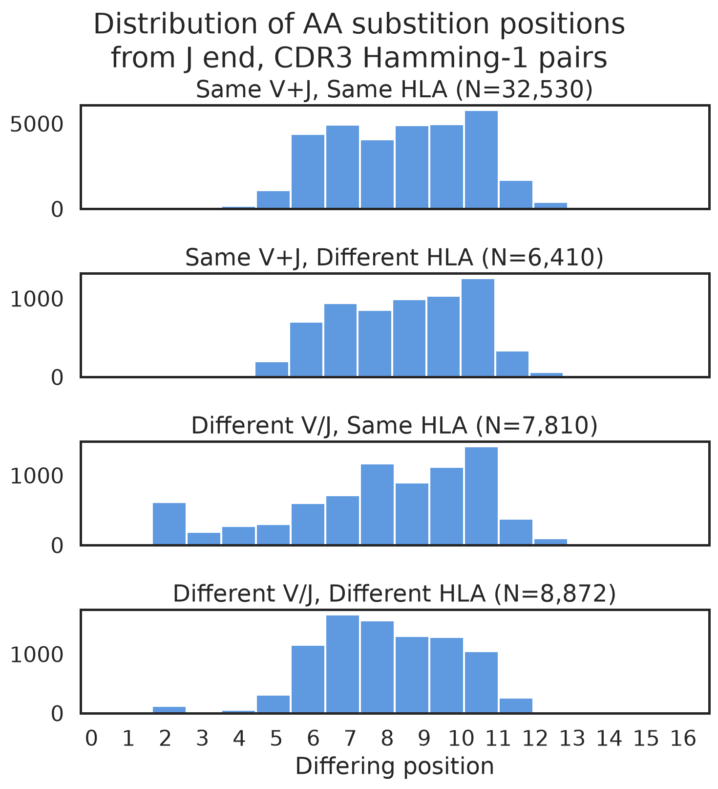
Let’s see if there’s a trend if we index the position from the J gene end instead of the V gene end.

hist_differing_positions(pdf_all_ham1_pairs, "differing_position_fromj", "J")

Nope. If we index from the J gene side, there’s no big outlier position that stands out like position 4 when indexed from the V gene side. Indexed from the J side, the distribution looks more like what I would naively expect to see: more substitutions in the middle of the CDR3 than at either end.

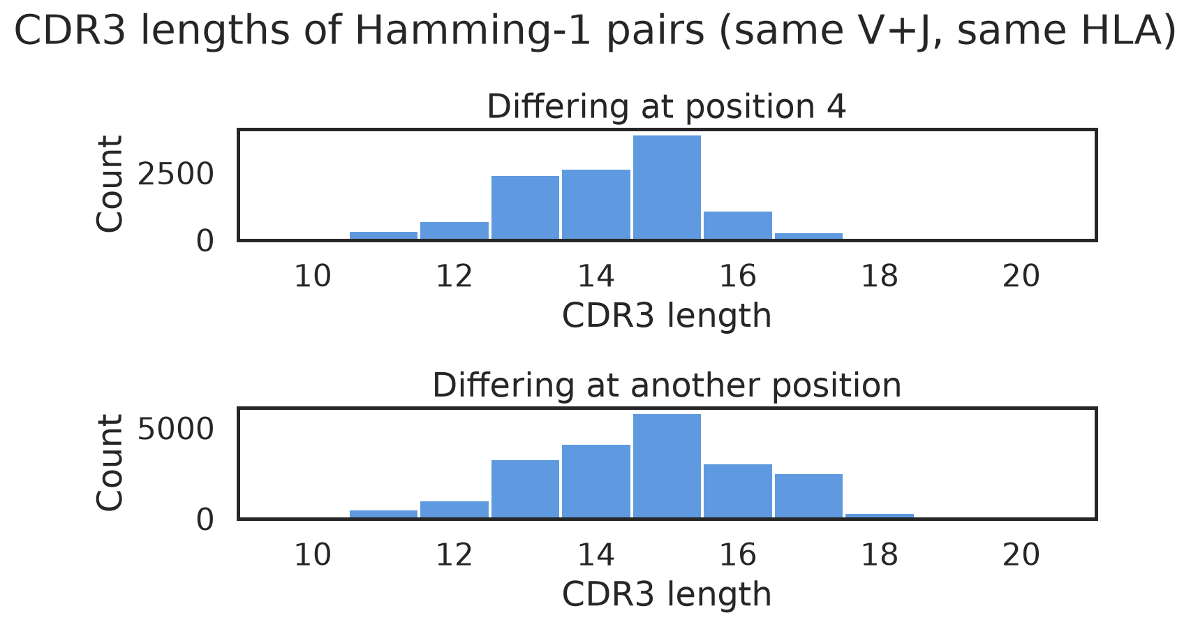
Let’s make sure that this trend isn’t dominated by a single huge sequence cluster, or something like that: let’s look at the distribution of CDR3 lengths of the Hamming-1 pairs that differ at position 4. If there’s an artefactual explanation, it should be dominated by a single length.

pdf_pos4_ham1_pairs_samehla_samevj = pdf_ham1_pairs_samehla_samevj[
    pdf_ham1_pairs_samehla_samevj.differing_position == 4]
pdf_notpos4_ham1_pairs_samehla_samevj = pdf_ham1_pairs_samehla_samevj[
    pdf_ham1_pairs_samehla_samevj.differing_position != 4]

f, (ax1, ax2) = plt.subplots(2, 1)
sns.histplot(pdf_pos4_ham1_pairs_samehla_samevj.cdr3_i.str.len(), bins=range(0, 30), discrete=True, ax=ax1)
ax1.set_title(f"Differing at position 4")
ax1.set_xlabel("CDR3 length")

sns.histplot(pdf_notpos4_ham1_pairs_samehla_samevj.cdr3_i.str.len(), bins=range(0, 30), discrete=True, ax=ax2)
ax2.set_title(f"Differing at another position")
ax2.set_xlabel("CDR3 length")

f.suptitle("CDR3 lengths of Hamming-1 pairs (same V+J, same HLA)", y=0.95)
f.tight_layout()

Nope! The distribution of CDR3 lengths for the pairs differing at position 4 is practically the same as the distribution for the pairs differing at other positions. So, the outsized proportion of pairs differing at position 4 isn’t explained by a single big sequence cluster.

Does the proportion of pairs differing at position 4 differ by HLA class association?

pdf_ham1_pairs_samehla_samevj["hla_class_i"] = pdf_ham1_pairs_samehla_samevj["hla_i"].apply(
    lambda x: "cii" if x.startswith("D") else "ci")
pdf_ham1_pairs_samehla_samevj["pos_4"] = pdf_ham1_pairs_samehla_samevj["differing_position"] == 4
pdf_ham1_pairs_samehla_samevj_ci = pdf_ham1_pairs_samehla_samevj[pdf_ham1_pairs_samehla_samevj.hla_class_i == "ci"]
pdf_ham1_pairs_samehla_samevj_cii = pdf_ham1_pairs_samehla_samevj[pdf_ham1_pairs_samehla_samevj.hla_class_i == "cii"]

proportion_ci_pos4 = sum(pdf_ham1_pairs_samehla_samevj_ci.pos_4) / len(pdf_ham1_pairs_samehla_samevj_ci)
proportion_cii_pos4 = sum(pdf_ham1_pairs_samehla_samevj_cii.pos_4) / len(pdf_ham1_pairs_samehla_samevj_cii)
print(f"Proportion of Hamming-1 pairs differing at position 4 by HLA class:")
print(f"Class I: {proportion_ci_pos4:.2%}")
print(f"Class II: {proportion_cii_pos4:.2%}")

Proportion of Hamming-1 pairs differing at position 4 by HLA class:
Class I: 34.13%
Class II: 35.94%

Nope! It’s nearly identical.

6 Does the distribution of differing positions differ by V gene?

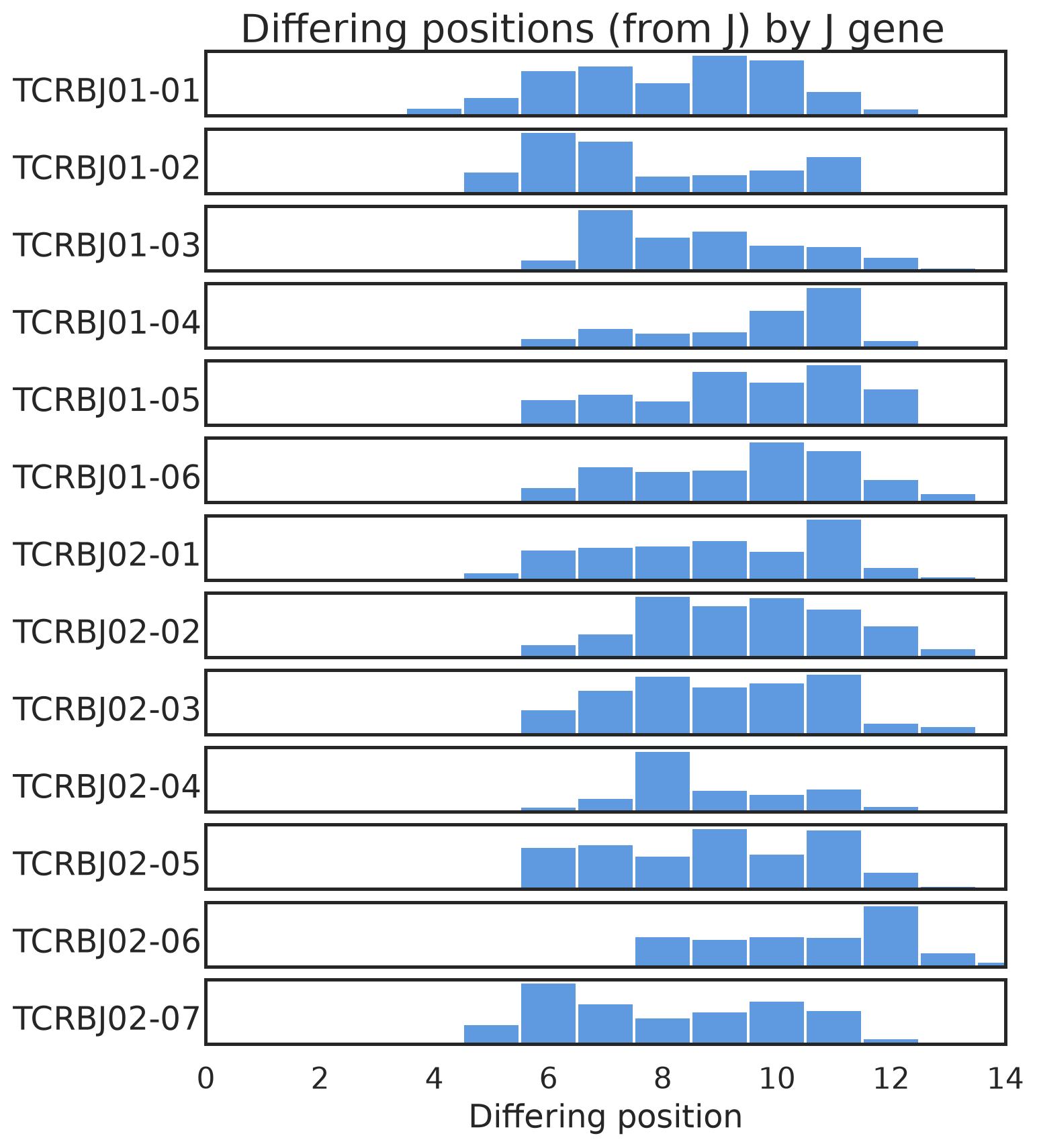
The most-differing position is fixed relative to the V gene but not the J gene. This suggests that it’s defined by the V-D boundary. That should vary by V gene, since different V genes extend different lengths past the CDR3 start.

If I recall correctly, those differences are consistent within V family, so let’s look at the distribution by V family.

pdf_ham1_pairs_samehla_samevj["vfamily"] = pdf_ham1_pairs_samehla_samevj["vgene_lower"].apply(
    lambda x: x.split("-")[0])
vfamilies = sorted(list(set(pdf_ham1_pairs_samehla_samevj.vfamily)))
f, axes = plt.subplots(len(vfamilies), 1, figsize=(8, 12))

rows = []
for i, vfamily in enumerate(vfamilies):
    pdf_vfamily = pdf_ham1_pairs_samehla_samevj[pdf_ham1_pairs_samehla_samevj.vfamily == vfamily]
    pdf_pos_counts = pdf_vfamily.differing_position.value_counts().reset_index()
    pdf_pos_counts.columns = ["differing_position", "count"]
    pdf_pos_counts = pdf_pos_counts.sort_values("count", ascending=False)
    n_max_pos = pdf_pos_counts["count"].iloc[0]
    prop_max_pos = n_max_pos / len(pdf_vfamily)
    max_pos = pdf_pos_counts["differing_position"].iloc[0]
    row = {
        "vfamily": vfamily,
        "n_pairs": len(pdf_vfamily),
        "max_pos": max_pos,
        "n_max_pos": n_max_pos,
        "prop_max_pos": prop_max_pos
    }
    rows.append(row)
    ax = axes[i]
    ax.set_xlim(0, max(pdf_ham1_pairs_samehla_samevj.differing_position) + 1)
    sns.histplot(pdf_vfamily.differing_position, discrete=True, ax=ax)
    ax.set_yticks([])
    if i < len(vfamilies) - 1:
        ax.set_xticks([])
    else:
        ax.set_xlabel("Differing position")

    ax.set_ylabel(vfamily, rotation=0, labelpad=45, y=0.1)
pdf_vfamily_maxpos_summary = pd.DataFrame(rows).sort_values("prop_max_pos", ascending=False)

f.suptitle("Distribution of differing positions by V family", y=0.91)
pass

Sure enough, most V families have the most swaps at position 4, but a few don’t:

pdf_vfamily_maxpos_summary[pdf_vfamily_maxpos_summary.max_pos != 4]

ⓘ	vfamily	n_pairs	max_pos	n_max_pos	prop_max_pos
2	TCRBV04	955	6	375	0.392670
12	TCRBV15	275	8	79	0.287273
14	TCRBV18	742	5	167	0.225067
17	TCRBV24	508	9	98	0.192913

TCRBV04 is dominated similarly by position 6. The rest are more spread out.

Is there a similar effect looking at J gene? Let’s see.

jgenes = sorted(list(set(pdf_ham1_pairs_samehla_samevj.jgene_i)))
f, axes = plt.subplots(len(jgenes), 1, figsize=(8, 10))

rows = []
for i, jgene in enumerate(jgenes):
    pdf_jgene = pdf_ham1_pairs_samehla_samevj[pdf_ham1_pairs_samehla_samevj.jgene_i == jgene]
    pdf_pos_counts = pdf_jgene.differing_position_fromj.value_counts().reset_index()
    pdf_pos_counts.columns = ["differing_position_fromj", "count"]
    pdf_pos_counts = pdf_pos_counts.sort_values("count", ascending=False)
    n_max_pos = pdf_pos_counts["count"].iloc[0]
    prop_max_pos = n_max_pos / len(pdf_jgene)
    max_pos = pdf_pos_counts["differing_position_fromj"].iloc[0]
    row = {
        "jgene": jgene,
        "n_pairs": len(pdf_jgene),
        "max_pos": max_pos,
        "n_max_pos": n_max_pos,
        "prop_max_pos": prop_max_pos
    }
    rows.append(row)
    ax = axes[i]
    ax.set_xlim(0, max(pdf_ham1_pairs_samehla_samevj.differing_position) + 1)
    sns.histplot(pdf_jgene.differing_position_fromj, discrete=True, ax=ax)
    ax.set_yticks([])
    if i < len(jgenes) - 1:
        ax.set_xticks([])
        ax.set_xlabel("")
    else:
        ax.set_xlabel("Differing position")
    ax.set_title("")
    ax.set_ylabel(jgene, rotation=0, labelpad=55, y=0.1)
pdf_gene_maxpos_summary = pd.DataFrame(rows).sort_values("prop_max_pos", ascending=False)

f.suptitle("Differing positions (from J) by J gene", y=0.91)
pass

Not really… no J gene has a single dominating position the way position 4 dominates for most V genes.

6.1 How to interpret/use this?

My working theory is that the position immediately after the V gene end is a “hotspot” for tolerated substitutions. That position is defined by the V gene and is usually position 4, but not always.

These observations could be incorporated into any function assessing distance between CDR3 sequences, for clustering or other purposes.

7 Amino acid pairs that tend to be swapped

Let’s look at the amino acids that are substituted and see if there are any patterns.

Since so many of the swaps are at position 4, and since amino acid prevalence varies dramatically by position, let’s just look at position 4 for demonstration.

Just to take V/J and HLA out of it, let’s look at just pairs with the same V, J and HLA association.

def heatmap_aa_pairs(pdf_ham1_pairs, title_suffix=""):
    pdf_aa_pairs = pdf_ham1_pairs.groupby(["aa_lower", "aa_higher"]).size().reset_index(name="count")
    pdf_aa_pairs = pdf_aa_pairs.sort_values(["aa_lower", "aa_higher"])
    pdf_aa_pairs_pivot = pdf_aa_pairs.pivot(index="aa_lower", columns="aa_higher", values="count").fillna(0)
    f, ax = plt.subplots()
    sns.heatmap(pdf_aa_pairs_pivot, cmap="YlGnBu")
    ax.set_title(f"Amino acid pairs at differing position" + title_suffix)
    # force all x and y ticks
    y_values = pdf_aa_pairs_pivot.index.values
    x_values = pdf_aa_pairs_pivot.columns.values
    ax.set_xticks([x + 0.5 for x in range(len(x_values))])
    ax.set_xticklabels(x_values)
    ax.set_yticks([x + 0.5 for x in range(len(y_values))])
    ax.set_yticklabels(y_values, rotation=0)
    ax.set_xlabel("'higher' AA")
    ax.set_ylabel("'lower' AA")

pdf_pos4_aapair_valuecounts = pdf_pos4_ham1_pairs_samehla_samevj["aa_pair"].value_counts().reset_index()

heatmap_aa_pairs(pdf_pos4_ham1_pairs_samehla_samevj, title_suffix="\n(same V+J+HLA, swap at position 4)")
pdf_pos4_aapair_valuecounts

ⓘaa_pair	count
LP	421
PS	387
AS	312
LS	306
AP	302
ST	290
FL	289
LR	258
LQ	256
GS	231
(161 more rows not shown)

There’s definitely a concentration of swaps in a few amino acid pairs. Looks like L tends to get swapped a lot, and P, and A.

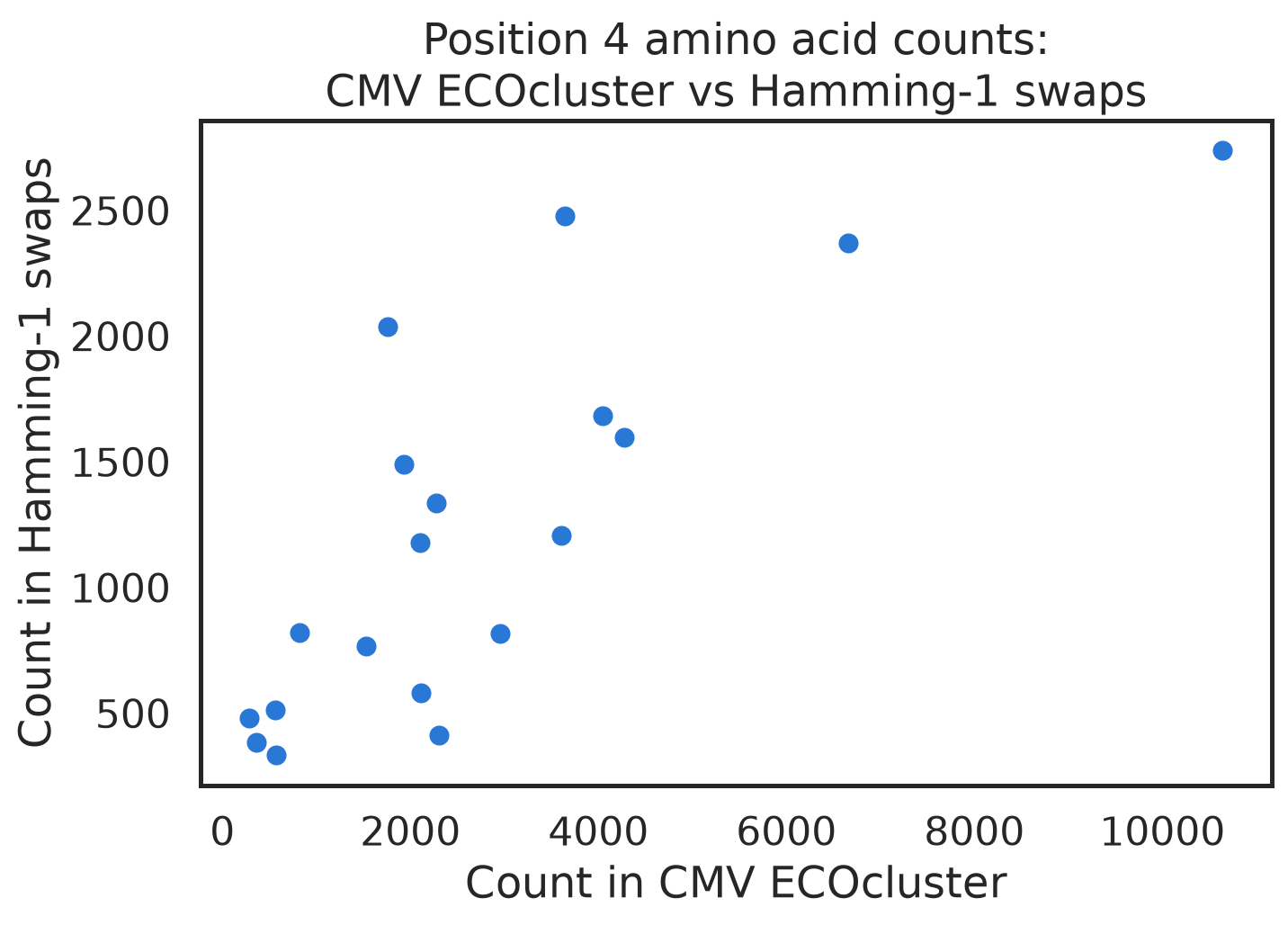
Of course, the different amino acids occur at different rates in the CMV ECOcluster TCRs. Are those concentrations of swaps statistically unlikely given the frequencies of amino acids at position 4 in the CMV ECOcluster? Let’s see.

# among all CMV ECOcluster TCRs, count the occurrences of each amino acid at position 4.
# Compare those with the presence in swaps
pdf_pos4_aa_valuecounts = pdf_cmv_ecocluster_2026["cdr3"].str[4].value_counts().reset_index()
pdf_pos4_aa_valuecounts.columns = ["aa", "count"]

pdf_aas_pos4_swaps_bothpositions = pd.concat([pdf_pos4_ham1_pairs_samehla_samevj["aa_lower"],
                                             pdf_pos4_ham1_pairs_samehla_samevj["aa_higher"]])
pdf_pos4swap_aa_counts = pdf_aas_pos4_swaps_bothpositions.value_counts().reset_index()
pdf_pos4swap_aa_counts.columns = ["aa", "count"]

pdf_pos4aas_cmveco_vs_swaps = pdf_pos4_aa_valuecounts.merge(pdf_pos4swap_aa_counts,
                                                            on="aa", how="outer", suffixes=("_cmveco", "_swaps")).fillna(0)

f, ax = plt.subplots()
sns.scatterplot(data=pdf_pos4aas_cmveco_vs_swaps, x="count_cmveco", y="count_swaps")
ax.set_title("Position 4 amino acid counts:\nCMV ECOcluster vs Hamming-1 swaps")
ax.set_ylabel("Count in Hamming-1 swaps")
ax.set_xlabel("Count in CMV ECOcluster")
pass

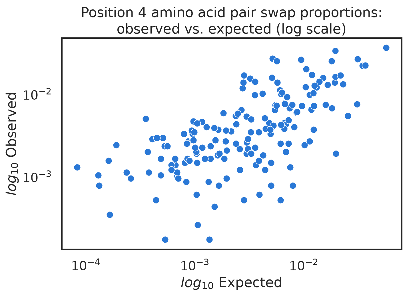
The more often an amino acid occurs at position 4, the more often it’s swapped. Let’s calculate the expected number of swaps involving each amino acid pair (given the frequency of each amino acid at position 4) and plot it against the observed number of swaps for each amino acid pair.

pdf_aapair_expectedcounts = pdf_pos4_aa_valuecounts.merge(pdf_pos4_aa_valuecounts, how="cross")
pdf_aapair_expectedcounts = pdf_aapair_expectedcounts[pdf_aapair_expectedcounts["aa_x"] != pdf_aapair_expectedcounts["aa_y"]]
pdf_aapair_expectedcounts["aa_pair"] = pdf_aapair_expectedcounts["aa_x"] + pdf_aapair_expectedcounts["aa_y"]
pdf_aapair_expectedcounts["aa_pair"] = pdf_aapair_expectedcounts["aa_pair"].apply(lambda x: "".join(sorted(x) ))
pdf_aapair_expectedcounts = pdf_aapair_expectedcounts.drop_duplicates("aa_pair")
pdf_aapair_expectedcounts["expected_count"] = pdf_aapair_expectedcounts["count_x"] * pdf_aapair_expectedcounts["count_y"]
pdf_aapair_expectedcounts["expected_proportion"] = pdf_aapair_expectedcounts["expected_count"] / pdf_aapair_expectedcounts["expected_count"].sum()

pdf_pos4_aapair_valuecounts["swap_proportion"] = pdf_pos4_aapair_valuecounts["count"] / pdf_pos4_aapair_valuecounts["count"].sum()
pdf_expected_actual_swap_proportions = pdf_aapair_expectedcounts[["aa_pair", "expected_count", "expected_proportion"]].merge(
    pdf_pos4_aapair_valuecounts[["aa_pair", "count", "swap_proportion"]], on="aa_pair", how="outer").fillna(0)
pdf_expected_actual_swap_proportions["actual_minus_expected"] = (
    pdf_expected_actual_swap_proportions["swap_proportion"] - pdf_expected_actual_swap_proportions["expected_proportion"])

f, ax = plt.subplots()
sns.scatterplot(data=pdf_expected_actual_swap_proportions, x="expected_proportion", y="swap_proportion")
ax.set_title("Position 4 amino acid pair swap proportions:\nobserved vs. expected (log scale)")
ax.set_ylabel("${log_{10}}$ Observed")
ax.set_xlabel("${log_{10}}$ Expected")
ax.set_yscale("log")
ax.set_xscale("log")

Again, the the trend is that, the more often we expect to see a swap, the more often we do see it.

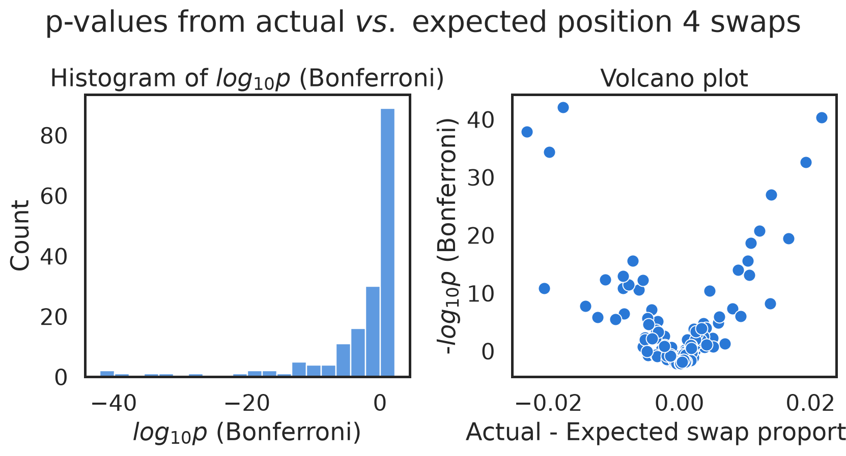
But there’s a lot of scatter around that trend. Are there AA pairs that are observed in swaps more or less often than we’d expect by chance? I’ll use Fisher’s Exact Test to look for statistically significant differences between the observed and expected swap counts for each amino acid pair, corrected for multiple testing using Bonferroni.

# test each pair of amino acids for whether the observed number of swaps is significantly different from the expected number of swaps,
# using a Fisher's exact test
from scipy.stats import fisher_exact
import numpy as np

pdf_expected_actual_swap_proportions["expected_count"] = pdf_expected_actual_swap_proportions["expected_proportion"] * pdf_pos4_aapair_valuecounts["count"].sum()
pdf_expected_actual_swap_proportions["observed_count"] = pdf_expected_actual_swap_proportions["swap_proportion"] * pdf_pos4_aapair_valuecounts["count"].sum()
pdf_expected_actual_swap_proportions["p_value"] = pdf_expected_actual_swap_proportions.apply(
    lambda row: fisher_exact([[row["observed_count"], row["expected_count"]],
                               [pdf_pos4_aapair_valuecounts["count"].sum() - row["observed_count"],
                                pdf_pos4_aapair_valuecounts["count"].sum() - row["expected_count"]]])[1], axis=1)
pdf_expected_actual_swap_proportions["p_value_bonf"] = pdf_expected_actual_swap_proportions["p_value"] * len(pdf_expected_actual_swap_proportions)

pdf_expected_actual_swap_proportions["log10_p_value_bonf"] = np.log10(pdf_expected_actual_swap_proportions["p_value_bonf"])

pdf_expected_actual_swap_proportions["neglog10_p_value_bonf"] = -pdf_expected_actual_swap_proportions["log10_p_value_bonf"]

f, (ax1, ax2) = plt.subplots(1, 2)
sns.histplot(pdf_expected_actual_swap_proportions.log10_p_value_bonf, bins=20, ax=ax1)
ax1.set_title("Histogram of $log_{10}p$ (Bonferroni)")
ax1.set_xlabel("$log_{10}p$ (Bonferroni)")


sns.scatterplot(x="actual_minus_expected", y="neglog10_p_value_bonf", data=pdf_expected_actual_swap_proportions, ax=ax2)
ax2.set_title("Volcano plot")
ax2.set_ylabel("-$log_{10}p$ (Bonferroni)")
ax2.set_xlabel("Actual - Expected swap proportion")
f.set_size_inches(9, 5)
f.suptitle("p-values from actual $vs.$ expected position 4 swaps", y=0.95)
f.tight_layout()

There certainly are! A large handful of swaps occur much more or less often than we’d expect to see by chance, given the amino acid frequencies at position 4. Let’s take a look at them:

print("Most overrepresented swaps:")
display(pdf_expected_actual_swap_proportions[pdf_expected_actual_swap_proportions.actual_minus_expected > 0].sort_values("p_value_bonf")[
        ["aa_pair", "p_value_bonf", "expected_proportion", "swap_proportion", "actual_minus_expected"]].head(10))
print("Most underrepresented swaps:")
display(pdf_expected_actual_swap_proportions[pdf_expected_actual_swap_proportions.actual_minus_expected < 0].sort_values("p_value_bonf")[
        ["aa_pair", "p_value_bonf", "expected_proportion", "swap_proportion", "actual_minus_expected"]].head(10))

Most overrepresented swaps:

ⓘ	aa_pair	p_value_bonf	expected_proportion	swap_proportion	actual_minus_expected
13	AS	4.666478e-41	0.005139	0.026866	0.021728
161	ST	2.703070e-33	0.005653	0.024972	0.019319
110	KR	1.008425e-27	0.002817	0.016792	0.013975
15	AV	1.719487e-21	0.003217	0.015414	0.012197
10	AP	3.500761e-20	0.009397	0.026005	0.016608
102	IV	2.286729e-19	0.002789	0.013692	0.010903
65	FY	2.532828e-16	0.003564	0.014036	0.010472
14	AT	9.276492e-15	0.002730	0.011711	0.008981
3	AG	7.168891e-14	0.005082	0.015758	0.010676
95	IM	4.165745e-11	0.000352	0.004994	0.004642

Most underrepresented swaps:

ⓘ	aa_pair	p_value_bonf	expected_proportion	swap_proportion	actual_minus_expected
24	DL	8.829449e-43	0.019653	0.001894	-0.017758
69	GL	1.466844e-38	0.030751	0.007492	-0.023259
40	EL	4.541473e-35	0.025253	0.005425	-0.019828
29	DR	2.687485e-16	0.007898	0.000775	-0.007123
149	PY	1.083707e-13	0.011272	0.002669	-0.008603
125	LY	4.454083e-13	0.018013	0.006717	-0.011297
79	GY	5.341731e-13	0.006096	0.000517	-0.005580
45	ER	3.449836e-12	0.010148	0.002411	-0.007737
27	DP	1.311395e-11	0.012298	0.003703	-0.008595
118	LP	1.370816e-11	0.056858	0.036252	-0.020605

So, e.g., even though L occurs in a lot of swaps, it actually occurs less often than we would expect by chance. And AS, ST, KR, etc., all occur far more often than we’d expect. ST and KR, at least, make a lot of sense, since they have very similar chemical properties.

We could put together a BLOSUM matrix from this kind of data (or multiple matrices for different parts of the sequence) and use it to score the similarity of CDR3 sequences with respect to pMHC binding. That should sound familiar! Anna Postovskaya did a very similar thing (tcrBLOSUM), using very different data. Her matrix also found AS, ST and KR to be well-tolerated.