Groups of poorly distinguished V and J genes

A few sets of V and J genes are often confused with each other. We should probably treat them as groups.

In ECOclusters, a TCR is defined as CDR3 amino acid sequence, V gene and J gene. That definition may be too restrictive for important applications of the CMV ECOcluster.

1 Takeaways from this post:

• In the CMV ECOcluster, we sometimes see the same CDR3 with different V or J genes
• Those mismatches are highly concentrated in a small number of groups of V genes and a single pair of J genes
  • This concentration is vanishingly unlikely by chance
• In nearly all such cases, the genes are in the same (V or J) family
  • The single exception isn’t nearly as well-supported as the rest
• We can and probably should treat those groups of V or J genes as equivalent when matching repertoire TCRs to the CMV ECOcluster
  • I built a library method to facilitate that kind of matching

2 Background

In bulk TCRB sequencing, it can be difficult to call v genes. Depending on the primers used, read length and the V gene of the TCR, there may be ambiguity.

ECOclusters are defined on a “TCR” definition consisting of V gene, J gene and CDR3 amino acid sequence. That definition might not be ideal if e.g. some pairs of V or J genes are often mistaken for each other. Let’s take a look at the CMV ECOcluster and see if we can find evidence that some groups of V or J genes should be combined.

3 Setup

# useful imports
import pandas as pd
import importlib
from cmvividly.data import access as cmv_access
from cmvividly.data.access import load_cmv_ecocluster_2026, load_cmv_ecocluster_2024
from matplotlib import pyplot as plt
from matplotlib_venn import venn2
import itables

itables.init_notebook_mode()


import seaborn as sns
from cmvividly.plots.style import set_style
set_style()

Load the CMV ECOcluster (2026 version). Add vfamily and jfamily fields.

# load the 2026 CMV ECOcluster.
pdf_cmv_ecocluster_2026 = load_cmv_ecocluster_2026()
pdf_cmv_ecocluster_2026["vfamily"] = pdf_cmv_ecocluster_2026.vgene.apply(lambda x: x.split("-")[0])
pdf_cmv_ecocluster_2026["jfamily"] = pdf_cmv_ecocluster_2026.jgene.apply(lambda x: x.split("-")[0])

4 Find pairs of TCRs with the same CDR3 sequence

When we see two TCRs with the same CDR3 in the CMV ECOcluster, my prior that they’re binding the same CMV peptide is very strong. Each TCR only occurs once, so any such pairs must have different V and/or J gene assignments.

Pairs of V genes or J genes that tend to show up with the same CDR3, over and over, may have trouble being distinguished by the V/J gene caller, or they may have similar pMHC binding characteristics. Let’s look for such pairs.

# identify cdr3 values that occur more than once
pdf_tcr_counts = pdf_cmv_ecocluster_2026['cdr3'].value_counts().reset_index()
multiocc_tcrs = pdf_tcr_counts[pdf_tcr_counts['count'] > 1]['cdr3'].tolist()
print(f"{len(multiocc_tcrs)} CDR3s occur more than once in the 2026 CMV ECOcluster")

1340 CDR3s occur more than once in the 2026 CMV ECOcluster

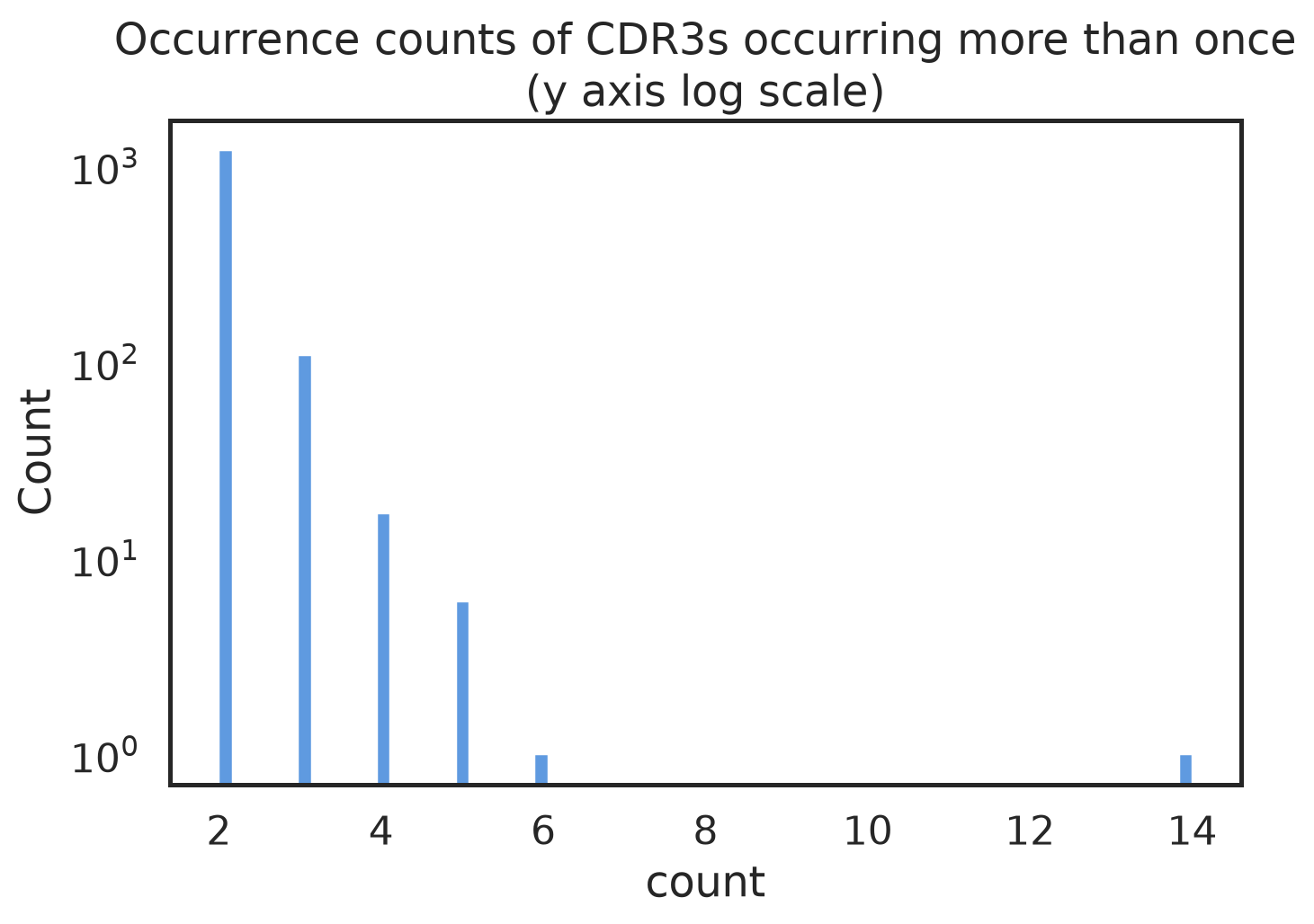
That’s a lot of multiply-occurring CDR3s! How many times does each occur?

f, ax = plt.subplots()
sns.histplot(pdf_cmv_ecocluster_2026[pdf_cmv_ecocluster_2026.cdr3.isin(multiocc_tcrs)].cdr3.value_counts())
ax.set_yscale("log")
ax.set_title("Occurrence counts of CDR3s occurring more than once\n(y axis log scale)")

Mostly just twice, but with a long tail. Let’s take a look at one that occurs several times.

pdf_cmv_ecocluster_2026[pdf_cmv_ecocluster_2026.cdr3 == multiocc_tcrs[1]][
    ["cdr3", "vgene", "jgene", "hla", "hla_cocluster"]]

ⓘ	cdr3	vgene	jgene	hla	hla_cocluster
4144	CASSWPGQGNTEAFF	TCRBV28-01	TCRBJ01-01	DRB3*02:02	h-DRB3_02_02-99
8645	CASSWPGQGNTEAFF	TCRBV18-01	TCRBJ01-01	DRB3*02:02	h-DRB3_02_02-99
12279	CASSWPGQGNTEAFF	TCRBV19-01	TCRBJ01-01	DRB3*02:02	h-DRB3_02_02-99
24754	CASSWPGQGNTEAFF	TCRBV14-01	TCRBJ01-01	DRB3*02:02	h-DRB3_02_02-99
35588	CASSWPGQGNTEAFF	TCRBV12-X	TCRBJ01-01	DRB3*02:02	h-DRB3_02_02-99
51378	CASSWPGQGNTEAFF	TCRBV07-06	TCRBJ01-01	DRB3*02:02	h-DRB3_02_02-99

Same J gene every time, same HLA association and HLA-COcluster… but 6 different V genes! CDR3s like that are rare, judging by the histogram above, but they do exist.

5 How often do we see the same CDR3 with different J genes?

pdf_cmv_ecocluster_2026_multicdr3 = pdf_cmv_ecocluster_2026[
    pdf_cmv_ecocluster_2026.cdr3.isin(multiocc_tcrs)]


pdf_cdr3_jgene_counts = pdf_cmv_ecocluster_2026_multicdr3.groupby(['cdr3']).agg({
    "jgene": pd.Series.nunique}).reset_index()
print(f"Max number of different J genes for a single CDR3: {max(pdf_cdr3_jgene_counts['jgene'])}. Breakdown:")
pdf_cdr3_jgene_counts["jgene"].value_counts().reset_index()

Max number of different J genes for a single CDR3: 3. Breakdown:

ⓘjgene	count
1	1298
2	41
3	1

So, it’s very rare, but in 41 cases there’s a pair of J genes with the same CDR3. In exactly one case, there are 3. Let’s look at that one.

cdr3_3_j_genes = pdf_cdr3_jgene_counts[pdf_cdr3_jgene_counts.jgene == 3]['cdr3'].tolist()[0]
pdf_cmv_ecocluster_2026_multicdr3[pdf_cmv_ecocluster_2026_multicdr3.cdr3 == cdr3_3_j_genes][
    ["cdr3", "vgene", "jgene", "hla", "hla_cocluster"]]

ⓘ	cdr3	vgene	jgene	hla	hla_cocluster
9446	CASSEATTQYF	TCRBV06-01	TCRBJ02-05	A*31:01	h-A_31_01-92
14051	CASSEATTQYF	TCRBV06-01	TCRBJ02-04	A*31:01	h-A_31_01-92
26518	CASSEATTQYF	TCRBV06-01	TCRBJ02-03	A*31:01	h-A_31_01-92

3 J genes, all in J family TCRBJ02, and the same V gene every time. Let’s take a more comprehensive look at those 41 J-gene pairs.

cdr3s_2_jgenes = pdf_cdr3_jgene_counts[pdf_cdr3_jgene_counts.jgene == 2].cdr3.tolist()
pdf_cmv_ecocluster_2026_twoj = pdf_cmv_ecocluster_2026_multicdr3[
    pdf_cmv_ecocluster_2026_multicdr3.cdr3.isin(cdr3s_2_jgenes)]

pdf_cdr3_jgene_lists = pdf_cmv_ecocluster_2026_twoj.groupby(['cdr3']).agg({
    "jgene": list}).reset_index()
pdf_cdr3_jgene_lists["jgene"] = [sorted(jgenes) for jgenes in pdf_cdr3_jgene_lists.jgene]
pdf_cdr3_jgene_lists["jgene_a"], pdf_cdr3_jgene_lists["jgene_b"] = zip(*pdf_cdr3_jgene_lists.jgene)
pdf_cdr3_jgene_lists[["jgene_a", "jgene_b"]].value_counts()

ⓘ		count
jgene_a	jgene_b
TCRBJ02-03	TCRBJ02-05	38
TCRBJ02-05	TCRBJ02-07	1
TCRBJ01-04	TCRBJ02-02	1
TCRBJ02-03	TCRBJ02-07	1

The same pair of Js accounting for 38 of 41 collisions among 13 J genes is vanishingly unlikely, on the face of it. But if those two are the most commonly-used J genes, then it’d be less unlikely. Let’s see:

pdf_cmv_ecocluster_2026.jgene.value_counts()

ⓘ	count
jgene
TCRBJ02-07	7195
TCRBJ02-01	6489
TCRBJ01-01	6026
TCRBJ01-02	5716
TCRBJ02-03	5505
TCRBJ02-05	4615
TCRBJ01-05	4263
TCRBJ02-02	3636
TCRBJ01-06	2771
TCRBJ01-04	2622
(3 more rows not shown)

Nope, J02-03 and J02-05 are middle of the pack. I could set up a statistical test (I’ll do that further down for V genes), but p would be effectively 0. But, to be thorough, let’s look at the CDR3s that have those two J genes. If they all represent just one sequence cluster, maybe there’s just a single binding solution that’s open to either J gene. If they’re very different, we’re more likely looking at a broad phenomenon.

for cdr3 in sorted(list(cdr3s_2_jgenes), key=lambda x: len(x)):
    print(cdr3)

CASGRGTQYF
CASSAGSAQYF
CASSAGSTQYF
CASSLERTQYF
CASSPGSAQYF
CASSSGSAQYF
CASSSGSGQYF
CASSSGSTQYF
CASTSGSTQYF
CASRGTVGTQYF
CASRSTVGTQYF
CASRTTVGTQYF
CASSDQGVTQYF
CASSELGVTQYF
CASSFRRQTQYF
CAWSVNREAQYF
CASSDDRRGTQYF
CASSEVGQGTQYF
CASSGGTSGTQYF
CASSIERGGTQYF
CASSLEAEGTQYF
CASSLEVRGTQYF
CASSLGLKGTQYF
CASSLWGAGTQYF
CASSPDRRGTQYF
CASSQRTGRELFF
CASSVAREETQYF
CASSVARGETQYF
CASSVARSETQYF
CSVVTSGRGTQYF
CASSLDAGGGTQYF
CASSLNRGEGTQYF
CASSPGQAGGTQYF
CASSPGQGQGTQYF
CASSPQGGPGTQYF
CASSQAGSLGTQYF
CATSDSTPGGTQYF
CSASPGLAVGTQYF
CASSPGQGARGTQYF
CASSQDRGTLLTQYF
CASSVGQGARGTQYF

That’s a wide variety of CDR3s. So, it seems likely that either:

• J gene caller is having trouble distinguishing between J02-03 and J02-05
• J02-03 and J02-05 often bind with an HLA molecule to present a similar binding surface

Either way, we should probably treat those two J genes as equivalent when we match these CMV ECOcluster TCRs to repertoires. If we see a CDR3 that matches, with the same V gene, but in the ECOcluster it uses J02-03 and in the repertoire it uses J02-05, we should probably consider them a match.

6 How often do we see the same CDR3 with different V genes?

pdf_cdr3_vgene_counts = pdf_cmv_ecocluster_2026_multicdr3.groupby(['cdr3']).agg({
    "vgene": pd.Series.nunique}).reset_index()
pdf_cdr3_multivgene_counts = pdf_cdr3_vgene_counts[
    pdf_cdr3_vgene_counts.vgene > 1]
n_cdr3s_multiv = len(pdf_cdr3_multivgene_counts)
print(f"CDR3s with multiple V genes: {n_cdr3s_multiv}")

cdr3s_multi_vgenes = pdf_cdr3_jgene_counts[pdf_cdr3_vgene_counts.vgene > 1].cdr3.tolist()
pdf_cmv_ecocluster_2026_multiv = pdf_cmv_ecocluster_2026_multicdr3[
    pdf_cmv_ecocluster_2026_multicdr3.cdr3.isin(cdr3s_multi_vgenes)]
n_tcrs_multivcdr3 = len(pdf_cmv_ecocluster_2026_multiv)
print(f"TCRs with multi-V CDR3s: {n_tcrs_multivcdr3} / {len(pdf_cmv_ecocluster_2026)} ({100 * n_tcrs_multivcdr3 / len(pdf_cmv_ecocluster_2026):.2f}%)")



print(f"Max number of different V genes for a single CDR3: {max(pdf_cdr3_multivgene_counts['vgene'])}. Breakdown:")
f, ax = plt.subplots()
sns.histplot(pdf_cdr3_multivgene_counts["vgene"], ax=ax)
ax.set_title("# different V genes for a single CDR3 with 2+")

CDR3s with multiple V genes: 1300
TCRs with multi-V CDR3s: 2776 / 52447 (5.29%)
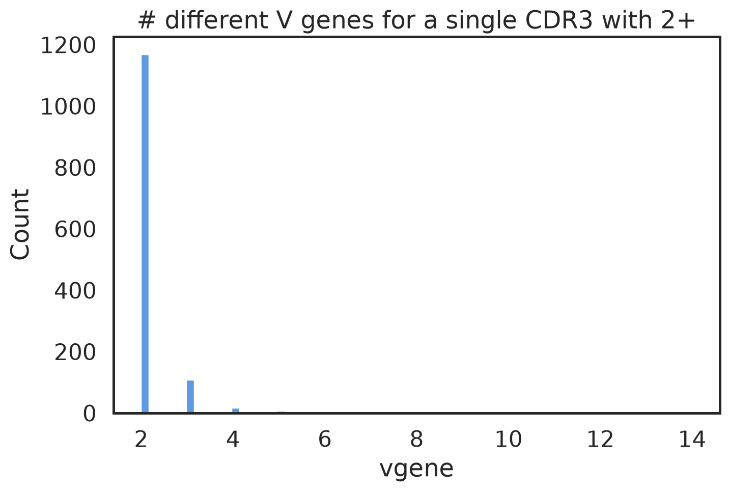
Max number of different V genes for a single CDR3: 14. Breakdown:

So, this is quite common! >5% of CMV ECOcluster TCRs are involved in one of these V-gene-mismatch cases. That suggests that dealing with this issue could increase sensitivity quite a bit when matching these TCRs to repertoires.

How often does this occur within vs. across V families?

# assemble the pairs
pdf_cdr3_vgene_lists = pdf_cmv_ecocluster_2026_multiv.groupby(['cdr3']).agg({
    "vgene": list}).reset_index()
pdf_cdr3_vgene_lists["vgene"] = [sorted(vgenes) for vgenes in pdf_cdr3_vgene_lists.vgene]
# explode all *pairs* of V genes for each CDR3.
pdf_all_cdr3_vgene_pairs = pdf_cdr3_vgene_lists.explode("vgene").merge(
    pdf_cdr3_vgene_lists.explode("vgene"), on="cdr3", suffixes=("_a", "_b"))
# pdf_all_cdr3_vgene_pairs contains two rows for each pair with different V genes.
# get rid of the one where vgene_a > vgene_b
pdf_cdr3_vgene_pairs = pdf_all_cdr3_vgene_pairs[
    (pdf_all_cdr3_vgene_pairs.vgene_a <= pdf_all_cdr3_vgene_pairs.vgene_b)]
# make vgene_a the lexicographically first of the two
pdf_cdr3_vgene_pairs["vgene_a"], pdf_cdr3_vgene_pairs["vgene_b"] = zip(*pdf_cdr3_vgene_pairs.apply(
    lambda x: sorted([x.vgene_a, x.vgene_b]), axis=1))
# drop any duplicates
pdf_cdr3_vgene_pairs = pdf_cdr3_vgene_pairs.drop_duplicates(["cdr3", "vgene_a", "vgene_b"])

#make a dataframe with just the different-V pairs
pdf_diff_cdr3_vgene_pairs = pdf_cdr3_vgene_pairs[
    pdf_cdr3_vgene_pairs.vgene_a < pdf_cdr3_vgene_pairs.vgene_b]


pdf_diff_cdr3_vgene_pairs["vfamily_a"] = pdf_diff_cdr3_vgene_pairs.vgene_a.apply(lambda x: x.split("-")[0])
pdf_diff_cdr3_vgene_pairs["vfamily_b"] = pdf_diff_cdr3_vgene_pairs.vgene_b.apply(lambda x: x.split("-")[0])
pdf_diff_cdr3_vgene_pairs["vfamily_agree"] = pdf_diff_cdr3_vgene_pairs.vfamily_a == pdf_diff_cdr3_vgene_pairs.vfamily_b
pdf_diff_cdr3_vgene_pairs["vfamily_agree"].value_counts().reset_index()

ⓘvfamily_agree	count
True	1131
False	626

pdf_diff_cdr3_vgene_pairs[pdf_diff_cdr3_vgene_pairs.cdr3 == "CSASPGLAVGTQYF"]

ⓘ	cdr3	vgene_a	vgene_b	vfamily_a	vfamily_b	vfamily_agree
5746	CSASPGLAVGTQYF	TCRBV20-01	TCRBV20-X	TCRBV20	TCRBV20	True

About 1/3 of the time, they have different V families. Let’s look at the top V gene pairs that have different V families.

pdf_diff_cdr3_vgene_pairs[~pdf_diff_cdr3_vgene_pairs.vfamily_agree][["vgene_a", "vgene_b"]].value_counts()

ⓘ		count
vgene_a	vgene_b
TCRBV05-01	TCRBV06-05	18
TCRBV07-02	TCRBV11-02	14
TCRBV05-01	TCRBV06-04	12
TCRBV07-08	TCRBV11-02	12
TCRBV07-02	TCRBV19-01	12
TCRBV11-02	TCRBV12-X	11
TCRBV06-05	TCRBV27-01	11
TCRBV06-04	TCRBV07-02	10
TCRBV02-01	TCRBV12-X	8
TCRBV05-05	TCRBV07-02	8
(282 more rows not shown)

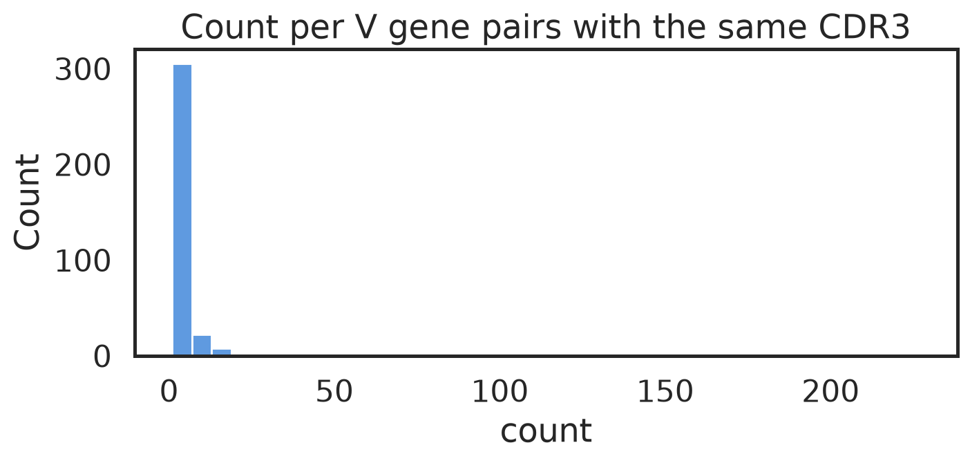
When these conflicts are cross-V-family, they’re not concentrated in a small number of V-gene or V-family pairs: the pair with the most conflicts has just 18 of 626. So, mismatch is primarily concentrated within a small number of pairs of V genes in the same V family.

Let’s see which V genes are most often involved in these cases.

pdf_vgene_pair_counts = pdf_diff_cdr3_vgene_pairs[["vgene_a", "vgene_b"]].value_counts().reset_index()

f, ax = plt.subplots()
sns.histplot(pdf_vgene_pair_counts["count"], ax=ax)
ax.set_title("Count per V gene pairs with the same CDR3")
f.set_size_inches(8, 3)

print("Top 10 V gene pairs with the same CDR3:")

pdf_vgene_pair_counts

Top 10 V gene pairs with the same CDR3:

ⓘvgene_a	vgene_b	count
TCRBV20-01	TCRBV20-X	227
TCRBV07-06	TCRBV07-X	139
TCRBV07-02	TCRBV07-03	90
TCRBV06-02	TCRBV06-02/06-03	68
TCRBV06-05	TCRBV06-X	61
TCRBV07-02	TCRBV07-X	53
TCRBV06-05	TCRBV06-06	49
TCRBV07-07	TCRBV07-X	43
TCRBV06-06	TCRBV06-X	33
TCRBV11-02	TCRBV11-X	31
(338 more rows not shown)

Several observations here:

• The top 15 V gene pairs (out of 348) are responsible for about half the mismatch
• It’s very concentrated in the top few V gene pairs, always in the same V family
• A lot of the pairs have a member ending in “-X”
  • That just means the V gene could only be resolved to the V-family level

Let’s see how often the pair contains an “-X” gene and then break out the “-X” and not-“-X” pairs separately.

pdf_diff_cdr3_vgene_pairs["has_x"] = pdf_diff_cdr3_vgene_pairs.apply(
    lambda x: "-X" in x.vgene_a or "-X" in x.vgene_b, axis=1)
display(pdf_diff_cdr3_vgene_pairs["has_x"].value_counts().reset_index())
print("No -X:")
display(pdf_diff_cdr3_vgene_pairs[~pdf_diff_cdr3_vgene_pairs.has_x][["vgene_a", "vgene_b"]].value_counts().reset_index())
print("Has -X:")
display(pdf_diff_cdr3_vgene_pairs[pdf_diff_cdr3_vgene_pairs.has_x][["vgene_a", "vgene_b"]].value_counts().reset_index())

ⓘhas_x	count
False	976
True	781

No -X:

ⓘvgene_a	vgene_b	count
TCRBV07-02	TCRBV07-03	90
TCRBV06-02	TCRBV06-02/06-03	68
TCRBV06-05	TCRBV06-06	49
TCRBV07-02	TCRBV07-08	30
TCRBV06-01	TCRBV06-05	26
TCRBV06-01	TCRBV06-06	22
TCRBV05-01	TCRBV06-05	18
TCRBV11-01	TCRBV11-02	18
TCRBV04-02	TCRBV04-03	17
TCRBV07-02	TCRBV11-02	14
(264 more rows not shown)

Has -X:

ⓘvgene_a	vgene_b	count
TCRBV20-01	TCRBV20-X	227
TCRBV07-06	TCRBV07-X	139
TCRBV06-05	TCRBV06-X	61
TCRBV07-02	TCRBV07-X	53
TCRBV07-07	TCRBV07-X	43
TCRBV06-06	TCRBV06-X	33
TCRBV11-02	TCRBV11-X	31
TCRBV07-08	TCRBV07-X	17
TCRBV06-02/06-03	TCRBV06-X	13
TCRBV06-01	TCRBV06-X	13
(64 more rows not shown)

7 Do all V genes get confused with [Vfamily]-X, or just some?

Is the observation here simply “sometimes we can’t discern V gene, only family”? Or is the mismatch restricted to a subset of genes per family?

Let’s look at the biggest offender, TCRBV20. How many TCRBV20 V genes are represented?

pdf_vgene_diffpair_counts_a = pdf_diff_cdr3_vgene_pairs.vgene_a.value_counts().reset_index()
pdf_vgene_diffpair_counts_a.columns = ["vgene", "count"]
pdf_vgene_diffpair_counts_b = pdf_diff_cdr3_vgene_pairs.vgene_b.value_counts().reset_index()
pdf_vgene_diffpair_counts_b.columns = ["vgene", "count"]
pdf_vgene_diffpair_counts_ab = pd.concat([pdf_vgene_diffpair_counts_a, pdf_vgene_diffpair_counts_b])
pdf_vgene_diffpair_counts = pdf_vgene_diffpair_counts_ab.groupby("vgene").agg({"count": "sum"}).reset_index().sort_values("count", ascending=False)
pdf_vgene_diffpair_counts.columns = ["vgene", "n_diff_pairs"]

pdf_vgene_counts = pdf_cmv_ecocluster_2026[["vgene", "vfamily"]].value_counts().reset_index()
pdf_vgene_counts.columns = ["vgene", "vfamily", "n_tcrs"]

pdf_vgene_counts_withdiffpairs = pdf_vgene_counts.merge(
    pdf_vgene_diffpair_counts, how="left", on="vgene").fillna(0)

pdf_vgene_counts_withdiffpairs["diffpairs_over_tcrs"] = (
    pdf_vgene_counts_withdiffpairs.n_diff_pairs / pdf_vgene_counts_withdiffpairs.n_tcrs)

pdf_vgene_counts_withdiffpairs[pdf_vgene_counts_withdiffpairs.vfamily == "TCRBV20"]

ⓘvgene	vfamily	n_tcrs	n_diff_pairs	diffpairs_over_tcrs
TCRBV20-X	TCRBV20	4018	227.0	0.056496
TCRBV20-01	TCRBV20	621	227.0	0.365539

Just one! And 100% of the mismatch involving TCRBV20-01 is with TCRBV20-X. So, in TCRBV20, it seems very clear we’d be better off just using V family.

How about TCRBV07?

pdf_vgene_counts_withdiffpairs[
    pdf_vgene_counts_withdiffpairs.vfamily == "TCRBV07"].sort_values("diffpairs_over_tcrs", ascending=False)

ⓘ	vgene	vfamily	n_tcrs	n_diff_pairs	diffpairs_over_tcrs
41	TCRBV07-X	TCRBV07	315	272.0	0.863492
43	TCRBV07-07	TCRBV07	222	84.0	0.378378
32	TCRBV07-06	TCRBV07	594	179.0	0.301347
28	TCRBV07-03	TCRBV07	665	129.0	0.193985
22	TCRBV07-08	TCRBV07	742	107.0	0.144205
5	TCRBV07-02	TCRBV07	2362	305.0	0.129128
9	TCRBV07-09	TCRBV07	1715	34.0	0.019825

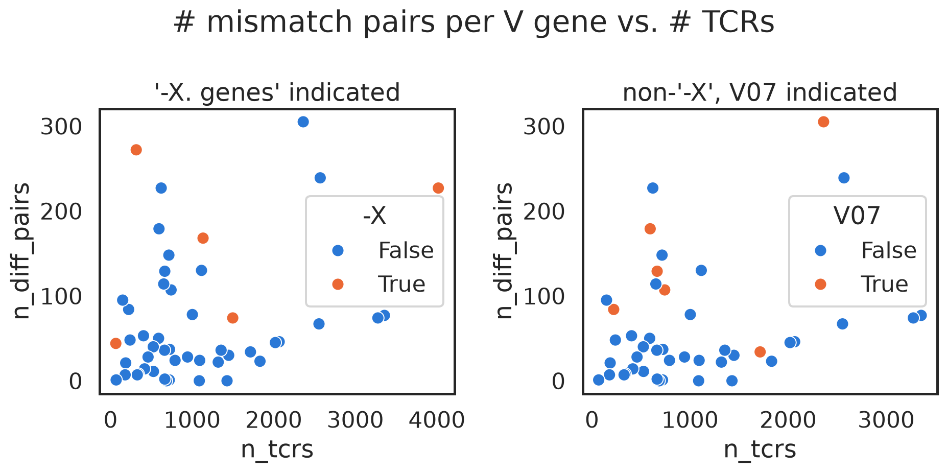
There are several V07 V genes represented. The relative number of TCRs is quite different from how often they show up in the mismatch pairs, though. Let’s place that within a broader context.

pdf_vgene_counts_withdiffpairs["-X"] = pdf_vgene_counts_withdiffpairs.vgene.str.endswith("-X")

f, (ax0, ax1) = plt.subplots(1, 2)
sns.scatterplot(x="n_tcrs", y="n_diff_pairs",
                data=pdf_vgene_counts_withdiffpairs, hue="-X", ax=ax0)
ax0.set_title("'-X. genes' indicated")

pdf_vgene_counts_withdiffpairs_nox = pdf_vgene_counts_withdiffpairs[~pdf_vgene_counts_withdiffpairs["-X"]]
pdf_vgene_counts_withdiffpairs_nox["V07"] = pdf_vgene_counts_withdiffpairs_nox.vgene.str.startswith("TCRBV07")

sns.scatterplot(x="n_tcrs", y="n_diff_pairs",
                data=pdf_vgene_counts_withdiffpairs_nox, hue="V07", ax=ax1)
ax1.set_title("non-'-X', V07 indicated")
f.suptitle("# mismatch pairs per V gene vs. # TCRs")
f.set_size_inches(10, 5)
f.tight_layout()

The “-X” genes (resolved at family level) are all involved in an outsized proportion of the mismatch pairs, as we’ve seen.

Most of the V07 genes are big outliers in how likely they are to be in mismatch pairs relative to their number of TCRs… but not TCRBV07-09. That V gene shows up quite often in the CMV ECOcluster but is rarely confused with another V gene.

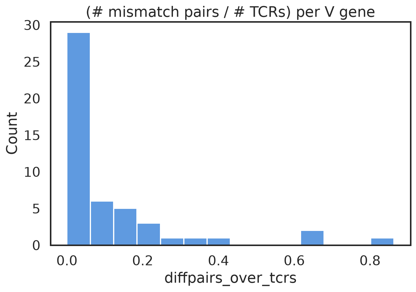
Let’s express the mismatch pairs as a fraction of the number of TCRs per V gene, and see if we’re looking at just a few outliers, or what.

f, ax = plt.subplots()
sns.histplot(pdf_vgene_counts_withdiffpairs["diffpairs_over_tcrs"])
ax.set_title("(# mismatch pairs / # TCRs) per V gene")


pdf_vgene_counts_withdiffpairs.sort_values("diffpairs_over_tcrs", ascending=False)[:10]

ⓘ	vgene	vfamily	n_tcrs	n_diff_pairs	diffpairs_over_tcrs	-X
41	TCRBV07-X	TCRBV07	315	272.0	0.863492	True
48	TCRBV11-X	TCRBV11	65	44.0	0.676923	True
46	TCRBV06-02	TCRBV06	149	95.0	0.637584	False
43	TCRBV07-07	TCRBV07	222	84.0	0.378378	False
31	TCRBV20-01	TCRBV20	621	227.0	0.365539	False
32	TCRBV07-06	TCRBV07	594	179.0	0.301347	False
25	TCRBV06-06	TCRBV06	715	148.0	0.206993	False
42	TCRBV11-01	TCRBV11	239	48.0	0.200837	False
28	TCRBV07-03	TCRBV07	665	129.0	0.193985	False
30	TCRBV06-02/06-03	TCRBV06	652	114.0	0.174847	False

Yep! We’re just looking at a handful of outlier pairs of V genes.

8 Adding a little statistical rigor

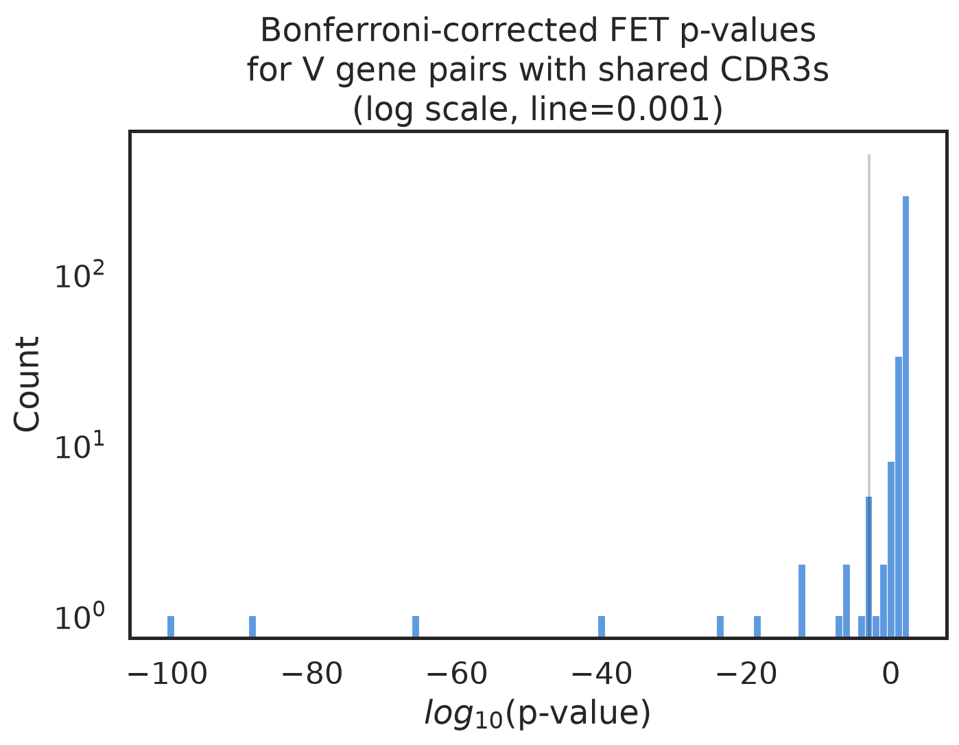
Let’s put some statistics around this. For each pair of V genes with any shared CDR3s, we can ask whether they’re enriched for shared CDR3s relative to their expected number of shared CDR3s (based on the count of CDR3-pair-members containing each member of the pair) if there was no enrichment. I’ll use a one-sided Fisher’s Exact Test for this, and then Bonferroni-correct for multiple testing.

from scipy.stats import fisher_exact
import numpy as np

def fisher_test_vgene_pair(row, pdf_cdr3_vgene_pairs):
    vgene_a = row['vgene_a']
    vgene_b = row['vgene_b']
    n_vgene_a = sum((pdf_cdr3_vgene_pairs.vgene_a == vgene_a) |
                    (pdf_cdr3_vgene_pairs.vgene_b == vgene_a))
    n_vgene_b = sum((pdf_cdr3_vgene_pairs.vgene_a == vgene_b) |
                    (pdf_cdr3_vgene_pairs.vgene_b == vgene_b))
    n_shared = row["count"]

    # calculate a Fisher's Exact Test p-value 
    n_total_pairs = len(pdf_cdr3_vgene_pairs)
    fisher_p = fisher_exact([[n_shared, n_vgene_a - n_shared],
                                 [n_vgene_b - n_shared, n_total_pairs - n_vgene_a - n_vgene_b + n_shared]],
                                alternative='greater')[1]
    return fisher_p

def test_all_vgene_pairs(pdf_vgenepair_counts_diff, pdf_cdr3_vgene_pairs):
    rows = []
    for _, row in pdf_vgenepair_counts_diff.iterrows():
        vgene_a = row['vgene_a']
        vgene_b = row['vgene_b']
        if vgene_a == vgene_b:
            continue  # Skip pairs where both V genes are the same

        n_vgene_a = sum((pdf_cdr3_vgene_pairs.vgene_a == vgene_a) |
                        (pdf_cdr3_vgene_pairs.vgene_b == vgene_a))
        n_vgene_b = sum((pdf_cdr3_vgene_pairs.vgene_a == vgene_b) |
                        (pdf_cdr3_vgene_pairs.vgene_b == vgene_b))
        n_shared = row["count"]

        # calculate a Fisher's Exact Test p-value 
        n_total_pairs = len(pdf_cdr3_vgene_pairs)
        fisher_p = fisher_exact([[n_shared, n_vgene_a - n_shared],
                                     [n_vgene_b - n_shared, n_total_pairs - n_vgene_a - n_vgene_b + n_shared]],
                                    alternative='greater')[1]

        rows.append({
            "vgene_a": vgene_a,
            "vgene_b": vgene_b,
            "n_vgene_a": n_vgene_a,
            "n_vgene_b": n_vgene_b,
            "n_shared": n_shared,
            "fisher_p": fisher_p
        })
    pdf_result = pd.DataFrame(rows).sort_values('fisher_p')
    pdf_result["p_fisher_bonf"] = pdf_result.fisher_p * len(pdf_result)
    # add a small epsilon when taking the log in case of underflow and p=0
    pdf_result["log10_p"] = np.log10(pdf_result.p_fisher_bonf + 1e-100)

    return pdf_result


pdf_vgenepair_counts = pdf_diff_cdr3_vgene_pairs[["vgene_a", "vgene_b"]].value_counts().reset_index()
pdf_vgenepair_counts_diff = pdf_vgenepair_counts[pdf_vgenepair_counts.vgene_a != pdf_vgenepair_counts.vgene_b]

pdf_vgenepair_pvalues = test_all_vgene_pairs(pdf_vgenepair_counts_diff, pdf_diff_cdr3_vgene_pairs)

thresh_bonf = .001


f, ax = plt.subplots()
sns.histplot(pdf_vgenepair_pvalues["log10_p"], bins=100)
# add vertical line at x=log10(thresh_bonf)
sns.lineplot(x=[np.log10(thresh_bonf), np.log10(thresh_bonf)], y=[0, 500], color="black", ax=ax,
            linestyle="dashed")
ax.set_yscale("log")
ax.set_title(f"Bonferroni-corrected FET p-values\nfor V gene pairs with shared CDR3s\n(log scale, line={thresh_bonf})")
ax.set_xlabel("${log}_{10}$(p-value)")

pdf_vgenepair_pvalues_signif = pdf_vgenepair_pvalues[
    pdf_vgenepair_pvalues.p_fisher_bonf < thresh_bonf]
print(f"{len(pdf_vgenepair_pvalues_signif)} V gene pairs survive Bonferroni correction at p<{thresh_bonf}")


pdf_vgenepair_pvalues.drop(columns=["log10_p"])

15 V gene pairs survive Bonferroni correction at p<0.001

ⓘ	vgene_a	vgene_b	n_vgene_a	n_vgene_b	n_shared	fisher_p	p_fisher_bonf
0	TCRBV20-01	TCRBV20-X	227	227	227	7.568311e-293	2.633772e-290
1	TCRBV07-06	TCRBV07-X	179	272	139	3.859408e-91	1.343074e-88
3	TCRBV06-02	TCRBV06-02/06-03	95	114	68	7.112069e-69	2.475000e-66
2	TCRBV07-02	TCRBV07-03	305	129	90	1.204637e-43	4.192137e-41
9	TCRBV11-02	TCRBV11-X	130	44	31	5.753066e-27	2.002067e-24
16	TCRBV04-02	TCRBV04-03	36	37	17	2.945112e-21	1.024899e-18
4	TCRBV06-05	TCRBV06-X	239	168	61	2.207718e-15	7.682860e-13
7	TCRBV07-07	TCRBV07-X	84	272	43	3.632770e-15	1.264204e-12
6	TCRBV06-05	TCRBV06-06	239	148	49	1.249498e-10	4.348253e-08
33	TCRBV04-01	TCRBV04-02	28	36	9	1.155829e-09	4.022284e-07
(338 more rows not shown)

So, being a little extra cautious, 15 pairs of V genes survive Bonferroni correction at p<0.001. All but one of those pairs are in the same V family. 6 involve a “-X” gene (V20, V07, V11 and V06).

One of those things is not like the others: {'TCRBV05-01', 'TCRBV06-04'}. Those two V genes are in different V families. Let’s take a closer look.

pdf_vgenepair_pvalues[(pdf_vgenepair_pvalues.vgene_a == "TCRBV05-01") & (pdf_vgenepair_pvalues.vgene_b == "TCRBV06-04")]

ⓘ	vgene_a	vgene_b	n_vgene_a	n_vgene_b	n_shared	fisher_p	p_fisher_bonf	log10_p
21	TCRBV05-01	TCRBV06-04	74	53	12	8.497749e-07	0.000296	-3.529117

That pair of V genes just barely survives Bonferroni correction at p<0.001. The number of shared CDR3s is 12, which is quite low among pairs that survive Bonferroni correction (see above).

As we did above with the J gene pair, let’s see what those 12 CDR3s look like.

n_5_1 = sum((pdf_cdr3_vgene_pairs.vgene_a == "TCRBV05-01") |
            (pdf_cdr3_vgene_pairs.vgene_b == "TCRBV05-01"))
n_6_4 = sum((pdf_cdr3_vgene_pairs.vgene_a == "TCRBV06-04") |
            (pdf_cdr3_vgene_pairs.vgene_b == "TCRBV06-04"))

pdf_5_1_6_4 = pdf_diff_cdr3_vgene_pairs[((pdf_diff_cdr3_vgene_pairs.vgene_a == "TCRBV05-01") & (pdf_diff_cdr3_vgene_pairs.vgene_b == "TCRBV06-04")) |
              ((pdf_diff_cdr3_vgene_pairs.vgene_a == "TCRBV06-04") & (pdf_diff_cdr3_vgene_pairs.vgene_b == "TCRBV05-01"))
]
for cdr3 in sorted(list(pdf_5_1_6_4.cdr3)):
    print(cdr3)

CASKKQGAADTQYF
CASRKQGAADTQYF
CASRKQGAGDTQYF
CASRKQGATDTQYF
CASRKQGSADTQYF
CASRKQGSSDTQYF
CASRKQGSTDTQYF
CASRKQGVTDTQYF
CASRLQGAGDTQYF
CASRLQGGTDTQYF
CASRLQGSTDTQYF
CASRLQGTTDTQYF

That looks like just a single binding solution with 12 TCRs: they’re all a single edit from another member of the group, i.e., a single connected component in a graph where edges are 1-edit differences.

That makes me nervous about combining those V genes: it could be that this one binding solution works with either of those V genes, but this binding solution is an outlier that doesn’t represent a general trend.

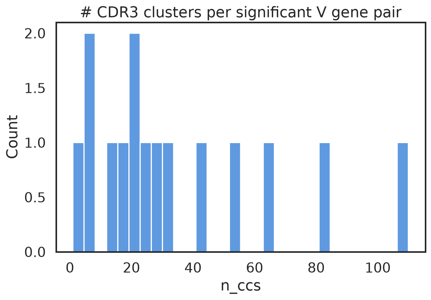
Let’s check all the other V gene pairs that survive Bonferroni correction: for each surviving V gene pair, build a graph on single edit distances and see how many connected components there are.

from cmvividly.data.hamming1_graph import build_seq_ham1_graph_and_extract_ccs

rows = []
for _, row in pdf_vgenepair_pvalues_signif.iterrows():
    vgene_a = row['vgene_a']
    vgene_b = row['vgene_b']
    pdf_pairs_this_pair = pdf_diff_cdr3_vgene_pairs[
        ((pdf_diff_cdr3_vgene_pairs.vgene_a == vgene_a) & (pdf_diff_cdr3_vgene_pairs.vgene_b == vgene_b)) |
        ((pdf_diff_cdr3_vgene_pairs.vgene_a == vgene_b) & (pdf_diff_cdr3_vgene_pairs.vgene_b == vgene_a))
    ]
    unique_cdr3_lengths = set(pdf_pairs_this_pair.cdr3.apply(len))
    
    # find connected components in a graph defined Hamming-1 distances between those CDR3s
    pdf_ccs = build_seq_ham1_graph_and_extract_ccs(pdf_pairs_this_pair)
    n_ccs = len(set(pdf_ccs.connected_component))

    rows.append({
        "vgene_a": vgene_a,
        "vgene_b": vgene_b,
        "n_shared_cdr3s": row["n_shared"],
        "unique_cdr3_lengths": unique_cdr3_lengths,
        "n_ccs": n_ccs
    })
pdf_vgenepair_cdr3_lengths = pd.DataFrame(rows).sort_values("n_shared_cdr3s", ascending=False)


f, ax = plt.subplots()
sns.histplot(pdf_vgenepair_cdr3_lengths["n_ccs"], ax=ax, bins=30)
ax.set_title("# CDR3 clusters per significant V gene pair")


pdf_vgenepair_cdr3_lengths.sort_values("n_ccs")

ⓘ	vgene_a	vgene_b	n_shared_cdr3s	unique_cdr3_lengths	n_ccs
12	TCRBV05-01	TCRBV06-04	12	{14}	1
13	TCRBV04-01	TCRBV04-03	7	{16, 18, 15}	5
9	TCRBV04-01	TCRBV04-02	9	{16, 17, 15}	8
10	TCRBV11-01	TCRBV11-02	18	{16, 13, 14, 15}	15
5	TCRBV04-02	TCRBV04-03	17	{12, 13, 14, 15, 16, 17, 18}	17
11	TCRBV06-01	TCRBV06-06	22	{11, 12, 13, 14, 15}	21
14	TCRBV06-06	TCRBV06-X	33	{12, 13, 14, 15, 16, 17, 19}	22
4	TCRBV11-02	TCRBV11-X	31	{11, 13, 14, 15, 16, 17, 18}	23
8	TCRBV06-05	TCRBV06-06	49	{12, 13, 14, 15, 16}	28
7	TCRBV07-07	TCRBV07-X	43	{12, 13, 14}	33
(5 more rows not shown)

Aha! All the other V gene pairs have at least 5 connected components represented. One has more than 100! So, {'TCRBV05-01', 'TCRBV06-04'} is the worst-supported pair in that sense, and the only cross-V-family pair.

I’ll strip that pair from the significant V gene pairs and move forward with the rest.

pdf_vgenepair_pvalues_retained = pdf_vgenepair_pvalues_signif[
    ~((pdf_vgenepair_pvalues_signif.vgene_a == "TCRBV05-01") & (pdf_vgenepair_pvalues_signif.vgene_b == "TCRBV06-04")) &
    ~((pdf_vgenepair_pvalues_signif.vgene_a == "TCRBV06-04") & (pdf_vgenepair_pvalues_signif.vgene_b == "TCRBV05-01"))
]
print(f"{len(pdf_vgenepair_pvalues_retained)} V gene pairs retained after removing TCRBV05-01/TCRBV06-04")

14 V gene pairs retained after removing TCRBV05-01/TCRBV06-04

9 Extract groups of V genes that should be considered indistinguishable

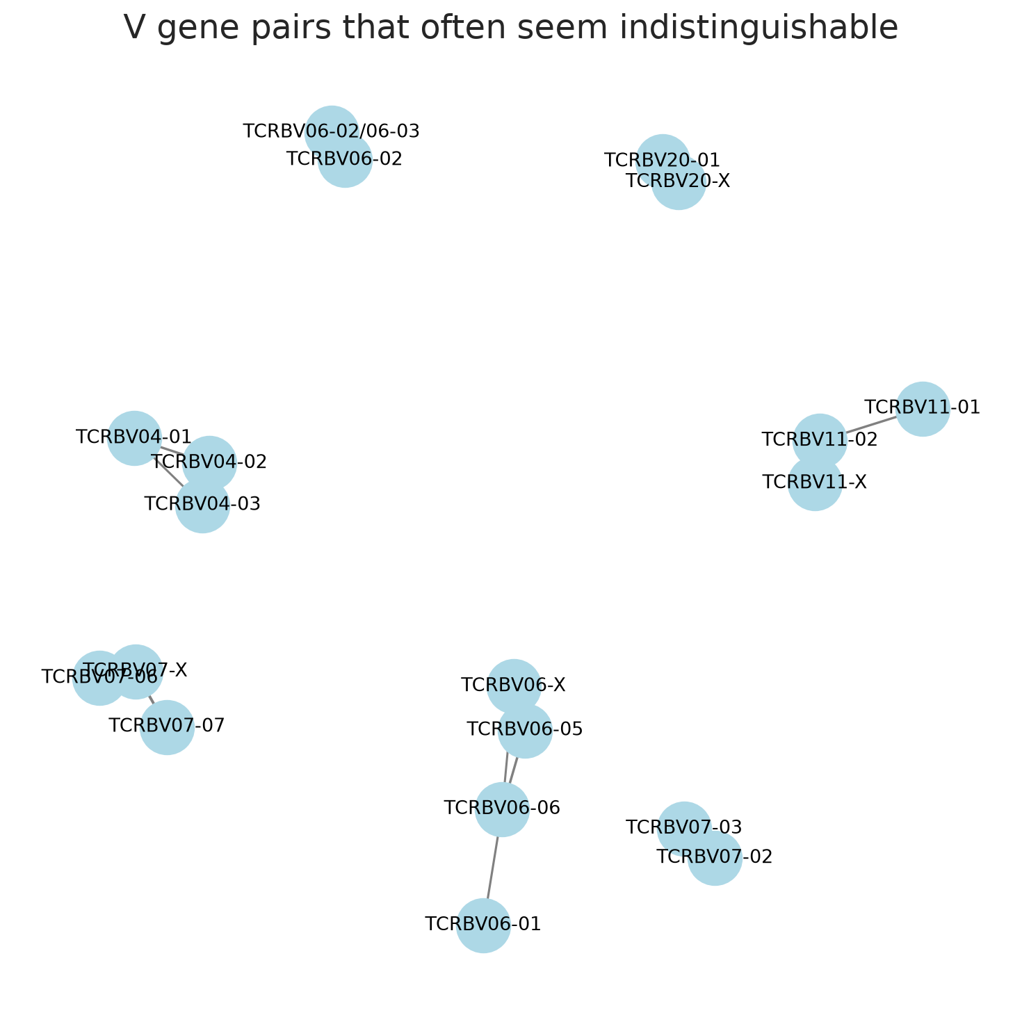
Most of these are small clusters of pairs, not just isolated pairs, so let’s visualize this.

# use networkx to visualize the V gene pairs that survive Bonferroni correction
from networkx import Graph
import networkx as nx

def build_pvalue_graph(pdf_vgenepair_pvalues_signif):
    G = Graph()
    for _, row in pdf_vgenepair_pvalues_signif.iterrows():
        G.add_edge(row['vgene_a'], row['vgene_b'], weight=-row['log10_p'])
    return G

def visualize_pvalue_graph(G):
    f, ax = plt.subplots()
    pos = nx.spring_layout(G, seed=42, k=0.8)
    edge_weights = [G[u][v]['weight'] for u, v in G.edges()]
    max_weight = max(edge_weights) if edge_weights else 1
    edge_widths = [1 + 4 * (w / max_weight) for w in edge_weights]

    nx.draw_networkx_nodes(G, pos, node_size=800, node_color="lightblue", ax=ax)
    nx.draw_networkx_labels(G, pos, font_size=10, ax=ax)
    nx.draw_networkx_edges(G, pos, width=edge_widths, edge_color="gray", ax=ax)

    edge_labels = {(u, v): f"{G[u][v]['weight']:.1f}" for u, v in G.edges()}

    ax.set_title("V gene pairs that often seem indistinguishable")
    ax.axis("off")
    f.set_size_inches(8, 8)
    f.tight_layout()

G = build_pvalue_graph(pdf_vgenepair_pvalues_retained)
visualize_pvalue_graph(G)

We’ve got groups sizes 2, 3 and 4. Let’s extract the connected components of that graph.

# extract connected components
vgene_clusters = list(nx.connected_components(G))
vgene_clusters

[{'TCRBV20-01', 'TCRBV20-X'},
 {'TCRBV07-06', 'TCRBV07-07', 'TCRBV07-X'},
 {'TCRBV06-02', 'TCRBV06-02/06-03'},
 {'TCRBV07-02', 'TCRBV07-03'},
 {'TCRBV11-01', 'TCRBV11-02', 'TCRBV11-X'},
 {'TCRBV04-01', 'TCRBV04-02', 'TCRBV04-03'},
 {'TCRBV06-01', 'TCRBV06-05', 'TCRBV06-06', 'TCRBV06-X'}]

10 Combining groups of V and J genes for improved repertoire matching

I think treating those pairs of V genes each as a single V gene is a pretty reasonable thing to do when applying the CMV ECOcluster TCRs to Adaptive data. Maybe even when using Adaptive data in general.

What does that mean practically? Well, if you’re working with Adaptive repertoire data, and you’ve got a TCR with one of those V genes that otherwise (CDR3 and J) matches to a CMV ECOcluster TCR with the other, you should probably treat it as a match.

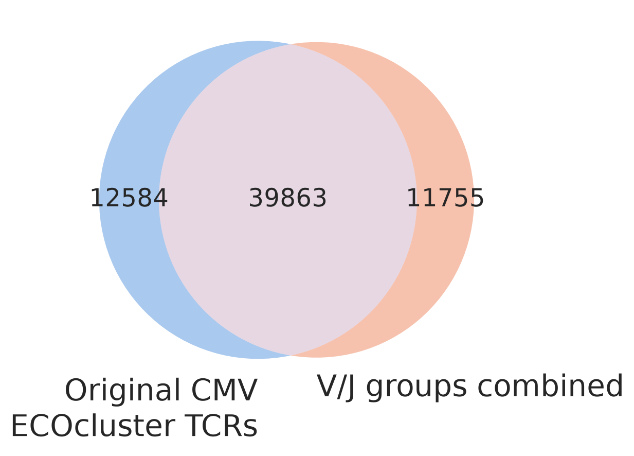
To facilitate that kind of matching, I made a library method, combine_indistinguishable_genes, that takes a dataframe of TCRs and returns a new dataframe with those genes combined using the mappings above: 7 groups of V genes and one group of two J genes.

Let’s apply that method to the CMV ECOclsuter TCRs and see how many TCRs we end up with.

from cmvividly.data.combine_v_j_groups import combine_indistinguishable_genes

pdf_cmv_ecocluster_2026_combinedvj = combine_indistinguishable_genes(
    pdf_cmv_ecocluster_2026, drop_original_gene_cols=False, retain_original_tcr=True).drop_duplicates("tcr")

print(f"Original CMV ECOcluster TCRs: {len(pdf_cmv_ecocluster_2026)}")
print(f"CMV ECOcluster TCRs after combining V/J groups: {len(pdf_cmv_ecocluster_2026_combinedvj)}")

from matplotlib_venn import venn2
venn2([set(pdf_cmv_ecocluster_2026.tcr), set(pdf_cmv_ecocluster_2026_combinedvj.tcr)],
      set_labels=("Original CMV\nECOcluster TCRs", "V/J groups combined"))

Original CMV ECOcluster TCRs: 52447
CMV ECOcluster TCRs after combining V/J groups: 51618

Bear in mind that you must also run the same V/J gene combination code on the repertoires you match the ECOcluster TCRs to! Otherwise, you’ll make fewer matches, rather than more.

We’ll see how this change to the matching strategy affects matching to repertoires in a later post.