The 2026 CMV ECOcluster has twice as many TCRs. What else changed?
Published
July 30, 2026
1 Why are there two versions of the CMV ECOcluster?
In 2024, we put out a preprint that made public an initial version of the CMV ECOcluster. In 2026, having rebuilt ECOclusters with more data and improved algorithms, we updated the ECOclusters preprint significantly and put a new version of the CMV ECOcluster in the supplemental data. The two versions both define sensitive, specific classifiers for CMV, but they’re very different from each other. Here, I’ll characterize the differences and try to explain them a bit.
Since anyone familiar with the 2024 CMV ECOcluster is likely to be a bit of an ECOclusters enthusiast, already, this post will get fairly far into some weeds.
2 Takeaways from this post:
The 2026 version has twice as many TCRs as 2024, but it’s missing most of the 2024 TCRs
The 2026 version is far more Class II-dominated (90% of TCRs vs. 65%)
In absolute terms, 2026 has many fewer Class I-associated TCRs than 2024
TCRs new in 2026 have much lower generation probability (pGen) than TCRs in both versions
The 2026 version likely had more statistical power to associate rarer TCRs
Almost a quarter of shared TCRs’ HLA allele associations disagree between versions
Almost none disagree on HLA class association
About half the TCRs “lost” in 2026 have at least one close sequence match among 2026 TCRs
That suggests many of them are missing for statistical/technical, not biological, reasons
The best way to use the 2024 and 2026 CMV ECOclusters may be to combine them, carefully
I took a first stab at that in a code block in this post (near the end)
I’ll explore the best way to combine them further in a future post
3 Setup
Basic imports.
Code
# useful importsimport pandas as pdimport seaborn as snsfrom cmvividly.data import access as cmv_accessfrom cmvividly.data.access import load_cmv_ecocluster_2026, load_cmv_ecocluster_2024from matplotlib import pyplot as pltfrom matplotlib_venn import venn2import itablesfrom cmvividly.plots.style import set_styleset_style()#statsfrom scipy.stats import mannwhitneyu
Load both versions of the CMV ECOcluster and count the rows.
Code
# load the 2024 CMV ECOcluster.pdf_cmv_ecocluster_2024 = load_cmv_ecocluster_2024()print(f"Rows in 2024 ECOcluster: {len(pdf_cmv_ecocluster_2024)}")# load the 2026 CMV ECOcluster.pdf_cmv_ecocluster_2026 = load_cmv_ecocluster_2026()print(f"Rows in 2026 ECOcluster: {len(pdf_cmv_ecocluster_2026)}")
Rows in 2024 ECOcluster: 26139
Rows in 2026 ECOcluster: 52447
First, a note: the 2024 CMV ECOcluster has some TCRs that occur multiple times, while the 2026 CMV ECOcluster does not:
Code
print(f"Max occurrences of a TCR in 2026:", pdf_cmv_ecocluster_2026["tcr"].value_counts().max())print(f"Occurrence count breakdown in 2024:")pdf_cmv_ecocluster_2024.tcr.value_counts().reset_index()["count"].value_counts()
Max occurrences of a TCR in 2026: 1
Occurrence count breakdown in 2024:
count
1    26073
2       33
Name: count, dtype: int64
That’s due to methodological differences in TCR-HLA allele association between 2024 and 2026. It’s pretty much a rounding error, but it’ll throw our accounting off slightly, so let’s deduplicate the 2024 version by TCR (taking an HLA association at random).
Code
pdf_cmv_ecocluster_2024_dedup = pdf_cmv_ecocluster_2024.drop_duplicates(subset=["tcr"])print(f"Rows in deduplicated 2024 dataframe: {len(pdf_cmv_ecocluster_2024_dedup)}")
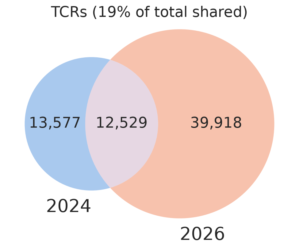
Wow! The 2026 ECOcluster is much bigger, but it loses half the TCRs from the 2024 version.
4.1 Break down TCRs in both versions by HLA class
Code
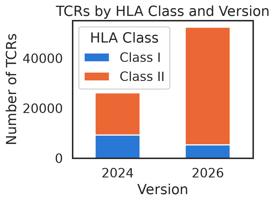
# build a 2x2 table: # of TCRs in 2024 where hla == "ci" and where hla == "cii", and same in 2026n_ci_2024 =sum(pdf_cmv_ecocluster_2024_dedup["hla_class"] =="ci")n_cii_2024 =sum(pdf_cmv_ecocluster_2024_dedup["hla_class"] =="cii")n_ci_2026 =sum(pdf_cmv_ecocluster_2026["hla_class"] =="ci")n_cii_2026 =sum(pdf_cmv_ecocluster_2026["hla_class"] =="cii")# Create a 2x2 tablepdf_hlaclass_by_version = pd.DataFrame({"Class I": [n_ci_2024, n_ci_2026],"Class II": [n_cii_2024, n_cii_2026],"% Class II": [n_cii_2024 / (n_ci_2024 + n_cii_2024) *100, n_cii_2026 / (n_ci_2026 + n_cii_2026) *100]}, index=["2024", "2026"])# make a stacked barplotf, ax = plt.subplots(figsize=(5, 4))pdf_hlaclass_by_version[["Class I", "Class II"]].plot(kind="bar", stacked=True, ax=ax)ax.set_xlabel("Version")ax.set_ylabel("Number of TCRs")ax.set_title("TCRs by HLA Class and Version")ax.legend(title="HLA Class")plt.xticks(rotation=0)plt.tight_layout()pdf_hlaclass_by_version
Class I
Class II
% Class II
2024
9242
16864
64.598177
2026
5323
47124
89.850706
The 2026 ECOcluster is 90% Class-II-associated TCRs, vs. 65% in 2024. That’s a big shift! And it’s consistent with the reported changes in HLA models between the two versions: as described in the preprint, Class II alleles tended to have dramatically more associated TCRs than Class II.
But, also, in absolute terms, the 2026 version actually has many fewer Class I-associated TCRs than the 2024 version did. That’s a bit of a surprise; I’ll look into that some more, further down.
4.2 Merge the two versions on TCR so we can compare them more specifically
Code
# first, add an hla_gene column so we can break things down by gene laterpdf_cmv_ecocluster_2024_dedup["hla_gene"] = pdf_cmv_ecocluster_2024_dedup.hla.apply(lambda x: x.split("*")[0])pdf_cmv_ecocluster_2026["hla_gene"] = pdf_cmv_ecocluster_2026.hla.apply(lambda x: x.split("*")[0])# set up an outer join on tcr, to build a dataframe that contains all TCRs in both ECOcluster versionsmerge_cols = ["tcr", "cdr3", "vgene", "jgene"]pdf_2024_merge = pdf_cmv_ecocluster_2024_dedup.copy()pdf_2024_merge["source_2024"] =Truepdf_2026_merge = pdf_cmv_ecocluster_2026.copy()pdf_2026_merge["source_2026"] =Truepdf_merged_tcr_outer = pdf_2024_merge.merge( pdf_2026_merge, on=merge_cols, how="outer", suffixes=("_2024", "_2026"), indicator=True,)# annotate each row with HLA class agreement and where the TCR came frompdf_merged_tcr_outer["hla_class_agree"] = ( pdf_merged_tcr_outer["hla_class_2024"] == pdf_merged_tcr_outer["hla_class_2026"])pdf_merged_tcr_outer["source"] = pdf_merged_tcr_outer["_merge"].map( {"left_only": "2024 only", "right_only": "2026 only", "both": "shared"})pdf_merged_tcr_outer["hla_class_sourced"] = pdf_merged_tcr_outer.apply(lambda row: row["hla_class_2024"] if row["source"] =="2024 only"else row["hla_class_2026"] if row["source"] =="2026 only"else row["hla_class_2024"] if row["hla_class_agree"]else"disagree", axis=1)pdf_merged_tcr_outer["source_2026"] = pdf_merged_tcr_outer.source_2026.fillna(False).astype(bool)pdf_merged_tcr_outer["source_2024"] = pdf_merged_tcr_outer.source_2024.fillna(False).astype(bool)print(f"TCRs in merged table: {len(pdf_merged_tcr_outer)}")
TCRs in merged table: 66024
4.2.1 Look at generation probability in the 2026 version
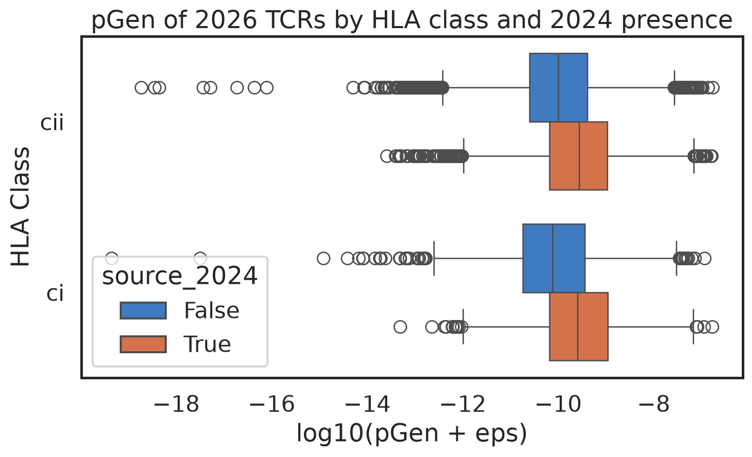
I don’t have convenient access to a pGen estimate for the 2024 version, but I can look at how it differs in the 2026 version by HLA class and by whether the TCR was in the 2024 version.
Code
pdf_2026_annot_2024 = pdf_merged_tcr_outer[pdf_merged_tcr_outer.source_2026 ==True]pdf_2026_annot_2024_droplowp = pdf_2026_annot_2024[pdf_2026_annot_2024.tcr_pgen >=1e-25]f, ax = plt.subplots()sns.boxplot(data=pdf_2026_annot_2024_droplowp, x="log10_tcr_pgen_eps", y="hla_class_2026", hue="source_2024", ax=ax, orient="horiz")ax.set_xlabel("log10(pGen + eps)")ax.set_ylabel("HLA Class")ax.set_title("pGen of 2026 TCRs by HLA class and 2024 presence")plt.tight_layout()pdf_2026_annot_2024_cii = pdf_2026_annot_2024[pdf_2026_annot_2024["hla_class_2026"] =="cii"]pdf_2026_annot_2024_ci = pdf_2026_annot_2024[pdf_2026_annot_2024["hla_class_2026"] =="ci"]higher_pgen_hlaclass ="Class II"if pdf_2026_annot_2024_cii["tcr_pgen"].mean() > pdf_2026_annot_2024_ci["tcr_pgen"].mean() else"Class I"mwu_p_hlaclass = mannwhitneyu( pdf_2026_annot_2024_cii["tcr_pgen"], pdf_2026_annot_2024_ci["tcr_pgen"],).pvaluemwu_p_cii = mannwhitneyu( pdf_2026_annot_2024_cii[pdf_2026_annot_2024_cii["source_2024"] ==True]["tcr_pgen"], pdf_2026_annot_2024_cii[pdf_2026_annot_2024_cii["source_2024"] ==False]["tcr_pgen"],).pvaluemwu_p_ci = mannwhitneyu( pdf_2026_annot_2024_ci[pdf_2026_annot_2024_ci["source_2024"] ==True]["tcr_pgen"], pdf_2026_annot_2024_ci[pdf_2026_annot_2024_ci["source_2024"] ==False]["tcr_pgen"],).pvalueprint(f"Two-sided Mann-Whitney U test p-values:")print(f"Between HLA classes: {mwu_p_hlaclass:.2e} ({higher_pgen_hlaclass} higher)")print(f"Within HLA class, 2024 vs. 2026: cii = {mwu_p_cii:.2e}, ci = {mwu_p_ci:.2e}")print("")print("(dropping very-low-pGen outliers for visibility)")
Two-sided Mann-Whitney U test p-values:
Between HLA classes: 1.22e-03 (Class I higher)
Within HLA class, 2024 vs. 2026: cii = 0.00e+00, ci = 1.84e-78

(dropping very-low-pGen outliers for visibility)
Overall, the Class II TCRs have slightly (and significantly) lower pGen. But the much bigger effect is that, in both HLA classes, the TCRs that are unique to the 2026 version have strongly lower pGen than the ones the two versions share. One way to interpret that is that the much larger dataset that built the new ECOclusters provides more statistical power to associate TCRs that are observed in fewer people.
That leaves the question: why are more than half of the 2024 TCRs missing from the 2026 version? I have a hypothesis that it’s not because they’re not actually CMV-specific. I’ll explore that further down in this post, and likely return to that question in a later post.
4.3 Look at the HLA class associations of TCRs in both versions, and unique to each
First let’s visualize how TCRs are either present or absent in each version, and associated with HLA Class I or Class II alleles in each version, with a Sankey plot.
Code
from cmvividly.plots.sankey import plot_sankeyplot_sankey(pdf_merged_tcr_outer.fillna("MISSING"), source_col="hla_class_2024", target_col="hla_class_2026")pass
That gives us a feel for what’s going on: HLA class is ~100% consistent when present in both versions, but there are a lot of TCRs just missing from one version. Almost all the new ones in 2026 are Class II, while the ones unique to 2024 are an even split.
Let’s look at that a little more precisely.
Code
source_hlaclass_breakdown = pd.crosstab(pdf_merged_tcr_outer.hla_class_sourced, pdf_merged_tcr_outer.source, margins=True)source_hlaclass_breakdown.loc["% Class I"] = (source_hlaclass_breakdown.loc["ci"] / source_hlaclass_breakdown.loc["All"] *100).map("{:.0f}%".format)source_hlaclass_breakdown.loc["% Class II"] = (source_hlaclass_breakdown.loc["cii"] / source_hlaclass_breakdown.loc["All"] *100).map("{:.0f}%".format)source_hlaclass_breakdown
source
2024 only
2026 only
shared
All
hla_class_sourced
ci
6940
3016
2301
12257
cii
6637
36902
10221
53760
disagree
0
0
7
7
All
13577
39918
12529
66024
% Class I
51%
8%
18%
19%
% Class II
49%
92%
82%
81%
There’s a lot in that table:
TCRs present in both versions are 82% Class II (between the 65% in 2024 and the 90% in 2026)
2024-only TCRs are about evenly split
2026-only TCRs are 92% Class II
Disagreements: almost none. 12,529 TCRs are in both versions, and all but 7 have the same HLA Class association.
5 Compare HLA alleles represented in the two versions
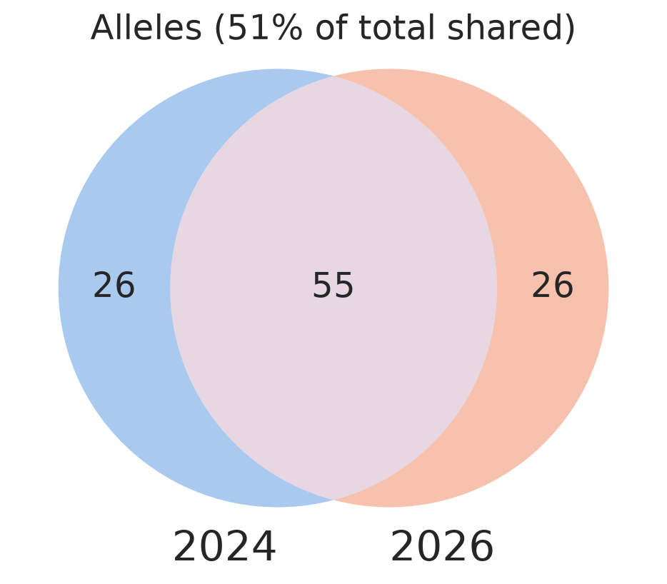
Let’s look at the specific alleles that drop out or show up in 2026 vs. 2024.
Code
def get_hlalist_by_gene(hlas) -> pd.DataFrame: genes =set([hla.split("*")[0] for hla in hlas]) gene_list_map = {gene: sorted([hla for hla in hlas if hla.startswith(gene)]) for gene inset([hla.split("*")[0] for hla in hlas])}return pd.DataFrame([{"gene": gene, "hlas": ", ".join(gene_list_map[gene])} for gene insorted(genes)])itables.init_notebook_mode()hlas_2024_only = hla_set_2024.difference(hla_set_2026)hlas_2026_only = hla_set_2026.difference(hla_set_2024)print("Alleles in 2024 only:")display(get_hlalist_by_gene(hlas_2024_only))print("Alleles in 2026 only:")display(get_hlalist_by_gene(hlas_2026_only))print(f"2026-only 'alleles' that are P groups: {sum([hla.endswith('P') for hla in hlas_2026_only])} of {len(hlas_2026_only)}")
Alleles in 2024 only:
Loading ITables v2.9.1 from the init_notebook_mode cell...
(need help?)
In the 2026 version, we combined several groups of HLA alleles in the same p group (alleles with the same binding domains) into a single model for each p group, after observing that they tended to have the same associated TCRs.
P groups gave us more statistical power to model alleles in 2026, but in the CMV ECOcluster they only replaced two 2024 alleles:
DRB1*14:54 -> DRB1*14:01P
DRB4*01:03 -> DRB4*01:01P
5.1 Do a lot of TCRs change HLA allele associations between versions?
Code
pdf_merged_tcr_inner = pdf_merged_tcr_outer[pdf_merged_tcr_outer["source"] =="shared"]pdf_merged_tcr_inner["hla_agree"] = pdf_merged_tcr_inner["hla_2024"] == pdf_merged_tcr_inner["hla_2026"]proportion_disagree = (pdf_merged_tcr_inner.hla_agree ==False).sum() /len(pdf_merged_tcr_inner)print(f"{proportion_disagree*100:.1f}% of TCR HLA associations disagree between versions")pdf_merged_tcr_inner.hla_agree.value_counts()
22.9% of TCR HLA associations disagree between versions
Loading ITables v2.9.1 from the init_notebook_mode cell...
(need help?)
That’s still a lot of disagreement at the HLA gene level! Let’s visualize it.
Code
from cmvividly.plots.sankey import plot_sankeyplot_sankey(pdf_merged_tcr_inner, source_col="hla_gene_2024", target_col="hla_gene_2026")pass
So, most of that movement is between DQA1 and DRB1, in both directions. That could be due to more LD between some of those alleles. Let’s get more granular and look at individual gene pairs.
Code
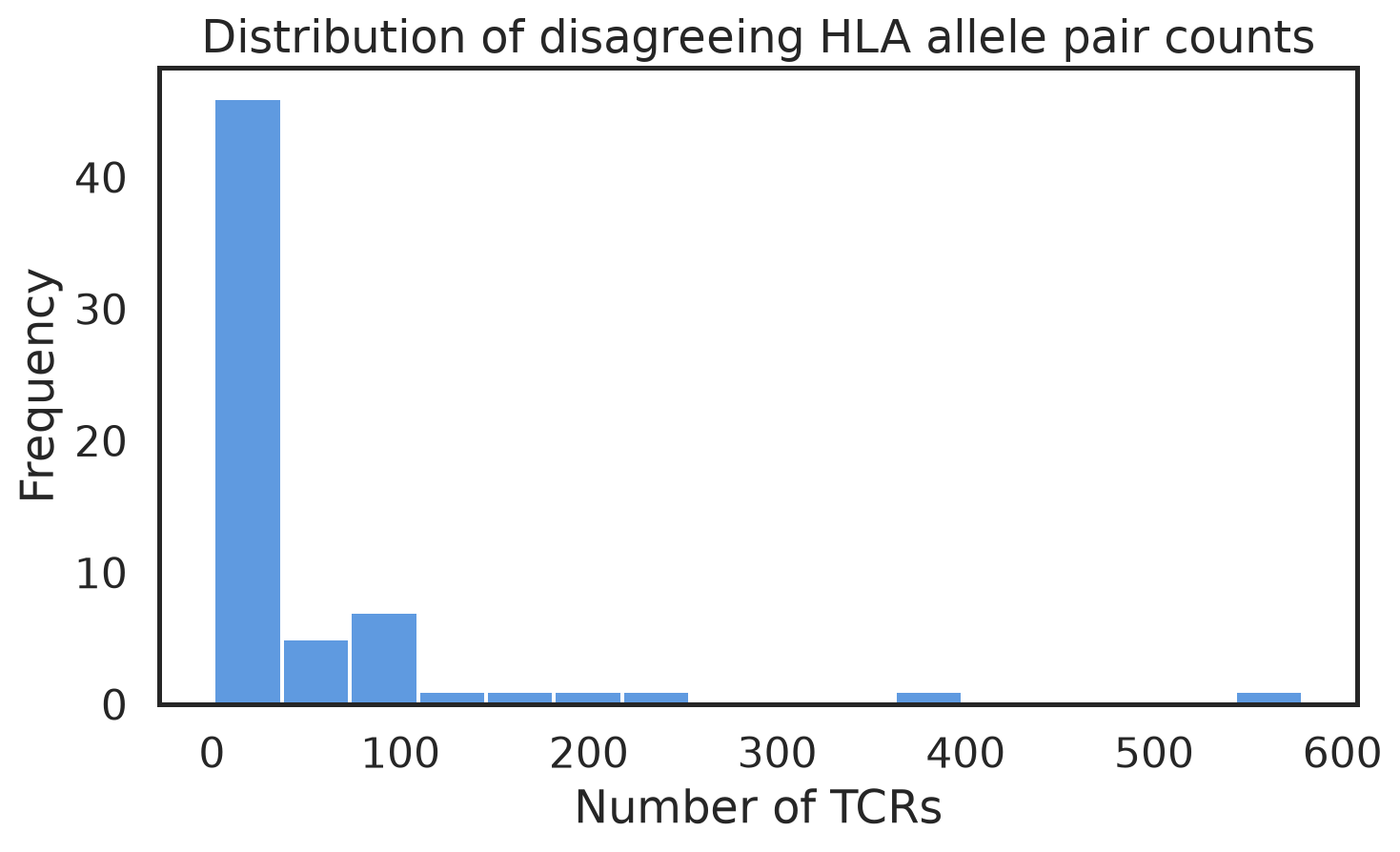
pdf_tcrs_disagree_hla = pdf_merged_tcr_inner[pdf_merged_tcr_inner.hla_agree ==False]pdf_disagreeing_allelepair_counts = pdf_tcrs_disagree_hla[["hla_2024", "hla_2026"]].value_counts().reset_index()f, ax = plt.subplots()sns.histplot(data=pdf_disagreeing_allelepair_counts, x="count", ax=ax)ax.set_xlabel("Number of TCRs")ax.set_ylabel("Frequency")ax.set_title("Distribution of disagreeing HLA allele pair counts")plt.tight_layout()print("Top pairs of disagreeing HLA alleles:")pdf_disagreeing_allelepair_counts[:8]
Top pairs of disagreeing HLA alleles:
Loading ITables v2.9.1 from the init_notebook_mode cell...
(need help?)
So, a handful of outlier allele pairs account for most of the allele association disagreement.
The third and sixth on the list is the easiest to explain: DRB1*14:54 -> DRB1*14:01P and DRB4*01:03 -> DRB4*01:01P, as I noted above.
The first one is the same heterodimer except DPB1*03:01 -> DPB1*104:01
Both those alleles are in TCE group 2, which suggests they might bind similar peptides
So, perhaps both heterodimers present peptides that those TCRs bind, and they’re simply getting assigned to different alleles in different versions due to statistical noise
I don’t have good explanations for the rest of the outliers. There could be some LD involved, or some pairs of alleles/heterodimers that bind similar peptides.
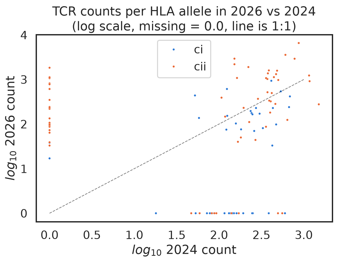
5.2 Have a look at TCR count per HLA allele in each version
We’ve summarized the biggest differences between the two versions of the CMV ECOcluster. But given that the 2024 ECOcluster has been available for two years and has been independently established as a sensitive, specific biomarker of CMV infection, it’s concerning that half those TCRs just go away in the new version. To put a point on it: the old one was good, the new one is good… but is some kind of hybrid better (or at least more comprehensive) than either?
I won’t answer that question completely in this post. In this post, I’ll just catalog what we’re “losing” in the 2026 ECOcluster and speculate about why. I plan to dig further in another post, using CMV-labeled repertoires.
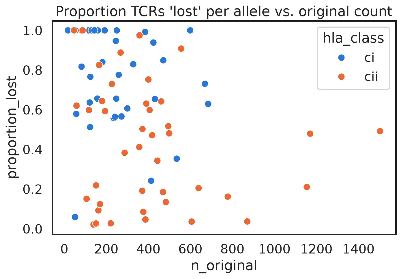
Let’s look at the HLA alleles that lost the most TCRs. Here, I don’t mean the TCR shows up in the 2026 ECOcluster associated with a different allele. I mean actually lost. We already learned above that those are about 50/50 Class I vs. Class II. How does that break down by allele?
Plot the proportion TCRs lost vs. the original TCR count.
Code
f, ax = plt.subplots()sns.scatterplot(x="n_original", y="proportion_lost", data=pdf_loss_summary, hue="hla_class")ax.set_title("Proportion TCRs 'lost' per allele vs. original count")
So, the biggest losers, in terms of proportion of TCRs lost, seem to be Class I alleles. That’s as expected, given that the 2026 ECOcluster is far more Class II-dominated and that, even though it’s much bigger overall, it actually has many fewer Class I-associated TCRs.
6.1 Are those “lost” TCRs sequence-similar to TCRs in the 2026 ECOcluster?
Highly sequence-similar TCRs tend to bind the same antigen. So, if many of those “lost” 2024 TCRs are sequence-similar to a 2026 TCR (I’ll define that here as same V gene, same J gene, same CDR3 length, one CDR3 edit), that’s strong evidence they shouldn’t have been lost. 1-Hamming doesn’t always mean same-antigen binding, but the additional evidence that it was CMV-associated in the 2024 version makes it pretty compelling.
Code
from cmvividly.data.hamming1_pairs import find_hamming1_pairs_same_vj# find all Hamming-1 pairs with the same v and j gene in the outer join between 2024 and 2026.# That's overkill, but that's the tooling I've built so far.pdf_ham1_pairs_all = find_hamming1_pairs_same_vj( pdf_merged_tcr_outer)pdf_ham1_pairs_all = ( pdf_ham1_pairs_all .drop(columns=["row_i", "row_j"]) .rename(columns={"tcr_i": "tcr_2024","tcr_j": "tcr_2026" }))# filter to just the ones present in 2024...pdf_ham1_pairs_in2024 = pdf_ham1_pairs_all[pdf_ham1_pairs_all.tcr_2024.isin(set(pdf_cmv_ecocluster_2024.tcr))]# ...with a match in 2026.pdf_ham1_pairs_in2024_pairin2026 = pdf_ham1_pairs_in2024[pdf_ham1_pairs_in2024.tcr_2026.isin(set(pdf_cmv_ecocluster_2026.tcr))]tcrs_2024_ham1_match_2026 =set(pdf_ham1_pairs_in2024_pairin2026.tcr_2024)lost_tcrs_2024 =set(pdf_cmv_ecocluster_2024_dedup[~pdf_cmv_ecocluster_2024_dedup.in_2026].tcr)lost_tcrs_2024_ham1_match_2026 = tcrs_2024_ham1_match_2026.intersection(lost_tcrs_2024)n_lost_2024 =len(lost_tcrs_2024)n_lost_with2026match =len(lost_tcrs_2024_ham1_match_2026)proportion_oflost_withmatch = n_lost_with2026match / n_lost_2024print(f"{n_lost_with2026match} of {n_lost_2024} 'lost' TCRs ({proportion_oflost_withmatch*100:.1f}%) have a Hamming-1 match in 2026")
2132 of 13577 'lost' TCRs (15.7%) have a Hamming-1 match in 2026
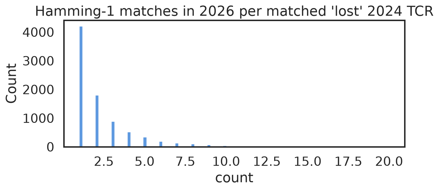
A lot of those “lost” TCRs have a match! Do they have just one? Lots of matches would be more evidence that they shouldn’t have been lost.
Code
pdf_losttcr_matchcounts = pdf_ham1_pairs_in2024_pairin2026.tcr_2024.value_counts().reset_index()f, ax = plt.subplots()sns.histplot(pdf_losttcr_matchcounts["count"])f.set_size_inches(8, 3)ax.set_title("Hamming-1 matches in 2026 per matched 'lost' 2024 TCR")
Almost half of the “lost” 2024 TCRs have at least 1 Hamming-1 match in 2026… and more than a quarter have 2+ matches… and some have as many as 20 Hamming-1 matches! That’s very strong evidence that some of those TCRs, at least, shouldn’t have been lost.
Why were they lost, then? Some ideas:
It could be due to a loss of statistical power, in one of two ways:
The samples used to build the 2026 ECOclusters were more numerous than the 2024 samples, but they weren’t a superset. It’s possible that some alleles had fewer allele+ donors in 2026.
Or maybe the mix of donor HLA alleles included more samples in incomplete LD with those alleles, making the HLA associations weaker.
Also, it was just a completely different clustering process, and a complicated one. Perhaps some of the drift is just due to different runs of HDBSCAN on different datasets, with no real underlying “reason”.
In any case, this analysis is a strong suggestion that many of those “lost” 2024 TCRs are actually CMV-specific.
7 Combining the two ECOclusters
The 2026 CMV ECOcluster is bigger and possibly “better”, overall. But the 2024 version has many TCRs and HLA alleles missing from 2026. If you’re applying the 2026 ECOcluster to repertoires, it’s worth trying the same analysis with the 2024 ECOcluster, and also combining them… carefully.
At the very least, we need to deal with the combining of groups of HLA alleles into p-group models that was done in the 2026 version but not in 2024. That allele mapping is in a big table in the supplementary materials for the 2026. The practical impact for the CMV ECOcluster is as described above:
DRB1*14:54 -> DRB1*14:01P
DRB4*01:03 -> DRB4*01:01P
In the code block below, I’ll take a quick stab at combining the two and dealing with those two p groups. This isn’t the final word on the best way to combine the two ECOclusters, so I won’t put this in library code yet.
Code
def combine_2024_2026_cmv_ecoclusters(pdf_cmv_ecocluster_2024, pdf_cmv_ecocluster_2026):"""This is a quick and dirty stab at combining the two ECOclusters. I'l button it up later, after seeing how the 2024 and 2026 TCRs behave in repertoires""" pdf_cmv_ecocluster_2024_formerge = pdf_cmv_ecocluster_2024_dedup.copy() pdf_cmv_ecocluster_2024_formerge["hla"] = ( pdf_cmv_ecocluster_2024_formerge.hla .replace("DRB1*14:54", "DRB1*14:01P") .replace("DRB4*01:03", "DRB4*01:01P") ) tcr_columns = ["cdr3", "vgene", "jgene"] pdf_combined_ecocluster = pdf_cmv_ecocluster_2024_formerge.merge( pdf_cmv_ecocluster_2026, on=tcr_columns, how="outer", suffixes=["_2024", "_2026"]) pdf_combined_ecocluster["hla"] = [ row["hla_2026"] ifisinstance(row["hla_2026"], str)else row["hla_2024"]for _, row in pdf_combined_ecocluster.iterrows() ]return pdf_combined_ecoclusterpdf_combined_ecocluster = combine_2024_2026_cmv_ecoclusters(pdf_cmv_ecocluster_2024, pdf_cmv_ecocluster_2026)
Let’s see how many TCRs and HLA alleles that combined ECOcluster comprises.
Code
n_tcrs =len(pdf_combined_ecocluster)n_hlas =len(set(pdf_combined_ecocluster.hla))print(f"Combined ECOcluster has {n_tcrs} TCRs associated with {n_hlas} HLA alleles")
Combined ECOcluster has 66024 TCRs associated with 105 HLA alleles
8 Making the best use of these two ECOclusters
In a future post, I plan to explore the ideas that the 2024-only TCRs are CMV-specific, and that the best way to use the two ECOclusters is to combine them, by seeing how those TCRs behave in CMV-labeled repertoires. I’ll also take a more formal stab at combining them in a way that deals with the differences in how they were built.