Basics

Download the CMV ECOcluster and have a look. Break down TCRs and HLA-COclusters by HLA allele and class.

Published

July 24, 2026

Download the CMV ECOcluster (using code from this repo) and have a look.

1 Takeaways from this post:

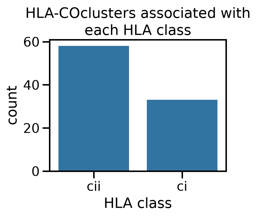
91 HLA-COclusters are associated with 81 HLA alleles
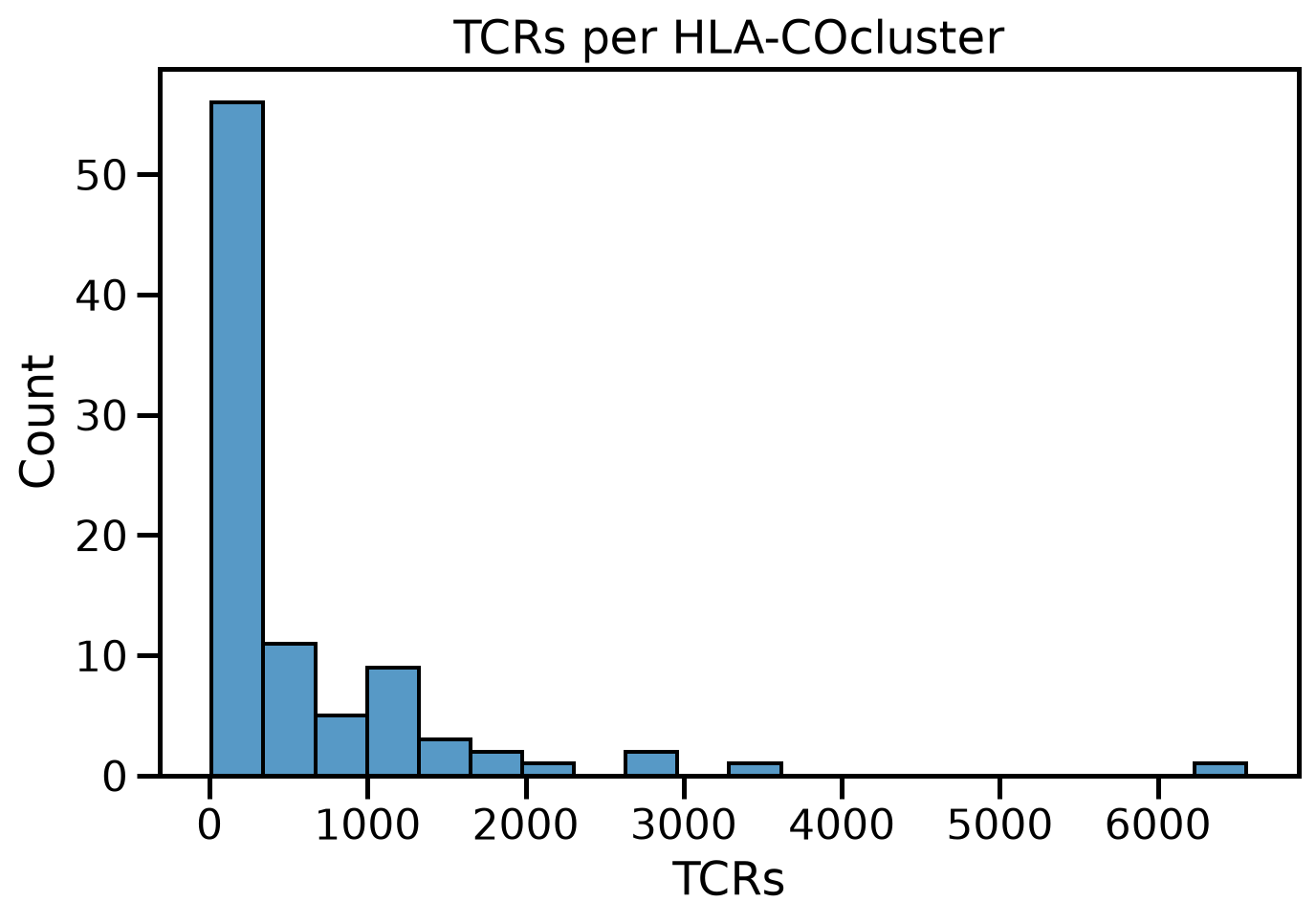
HLA-COclusters range in size from 14 to 6,562 TCRs
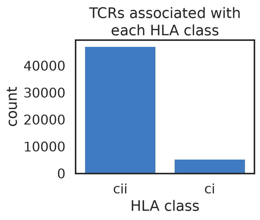
More TCRs are associated with Class II alleles than Class I, in bigger HLA-COclusters
A handful of alleles have more than one HLA-COcluster. They’re almost all Class I.
Class I TCRs have slightly but significantly higher pGen than Class II TCRs
- maybe due to greater statistical power in more-prevalent Class II alleles

2 Setup

Basic imports for data manipulation and plotting.

Code

# basic imports
import pandas as pd
from matplotlib import pyplot as plt
import seaborn as sns

# make plots look nice
from cmvividly.plots.style import set_style
set_style()

# make tables look nice and be interactive.
# itables can be a little fiddly, so just comment this out if it gives trouble
import itables
itables.init_notebook_mode()

# statistics
from scipy.stats import mannwhitneyu

init_notebook_modetrusted

Reminder before we get started: HLA-COclusters are subclusters of ECOclusters that are each associated with a single HLA-allele. ECOclusters are built by clustering the HLA-COclusters, by breadth correlation in repertoires, across HLA alleles.

3 Load the 2026 CMV ECOcluster

Load the dataset and display a sample of the rows (you can sort on the columns and search for values). The loader method I’m using adds a few extra columns.

Code

# load the CMV ECOcluster, downloading if not already downloaded.
from cmvividly.data.access import load_cmv_ecocluster_2026
pdf_cmv_ecocluster_2026 = load_cmv_ecocluster_2026()
pdf_cmv_ecocluster_2026

^ⓘtcr	cdr3	vgene	jgene	hla	hla_class	tcr_pgen	log10_tcr_pgen_eps	hla_cocluster	hla_cocluster_npos_hlamatch	hla_cocluster_nneg_hlamatch	hla_cocluster_auroc_hlaaware	hla_cocluster_auroc_hlaunaware
CASSLSGTGGWNEQFF+TCRBV07-02+TCRBJ02-01	CASSLSGTGGWNEQFF	TCRBV07-02	TCRBJ02-01	DRB1*07:01	cii	7.440500e-12	-11.128398	h-DRB1_07_01-718	11	19	0.961722	0.524297
CASSKQGANGYTF+TCRBV06-05+TCRBJ01-02	CASSKQGANGYTF	TCRBV06-05	TCRBJ01-02	DRB1*07:01	cii	3.790160e-10	-9.421343	h-DRB1_07_01-718	11	19	0.961722	0.524297
CASSIATGGAGYTF+TCRBV19-01+TCRBJ01-02	CASSIATGGAGYTF	TCRBV19-01	TCRBJ01-02	DRB1*07:01	cii	4.474897e-10	-9.349217	h-DRB1_07_01-718	11	19	0.961722	0.524297
CASSHFGTGGNTEAFF+TCRBV05-06+TCRBJ01-01	CASSHFGTGGNTEAFF	TCRBV05-06	TCRBJ01-01	DRB1*07:01	cii	1.609166e-11	-10.793399	h-DRB1_07_01-718	11	19	0.961722	0.524297
CASSLSRVAEQYF+TCRBV07-06+TCRBJ02-07	CASSLSRVAEQYF	TCRBV07-06	TCRBJ02-07	DRB1*07:01	cii	1.104376e-10	-9.956883	h-DRB1_07_01-718	11	19	0.961722	0.524297
CASKLQGAGDTQYF+TCRBV05-01+TCRBJ02-03	CASKLQGAGDTQYF	TCRBV05-01	TCRBJ02-03	DRB1*07:01	cii	1.100671e-11	-10.958342	h-DRB1_07_01-718	11	19	0.961722	0.524297
CAISATGTSGYEQYF+TCRBV10-03+TCRBJ02-07	CAISATGTSGYEQYF	TCRBV10-03	TCRBJ02-07	DQA101:05+DQB105:01	cii	2.586698e-10	-9.587254	h-DQA1_01_05_DQB1_05_01-588	1	0	NaN	0.595340
CASSYQGALGYTF+TCRBV06-05+TCRBJ01-02	CASSYQGALGYTF	TCRBV06-05	TCRBJ01-02	DRB1*07:01	cii	2.056430e-09	-8.686886	h-DRB1_07_01-718	11	19	0.961722	0.524297
CASSLAASGGTGELFF+TCRBV07-02+TCRBJ02-02	CASSLAASGGTGELFF	TCRBV07-02	TCRBJ02-02	DRB1*07:01	cii	2.961685e-10	-9.528461	h-DRB1_07_01-718	11	19	0.961722	0.524297
CSARVRLASAGELFF+TCRBV20-X+TCRBJ02-02	CSARVRLASAGELFF	TCRBV20-X	TCRBJ02-02	DRB1*07:01	cii	3.166421e-11	-10.499431	h-DRB1_07_01-718	11	19	0.961722	0.524297
(52,437 more rows not shown)

4 What are all those columns?

Most of the columns are as described in our preprint:

column	description
tcr	TCRB CDR3 amino acid sequence, V gene and J gene, delimited by ‘+’
hla	the HLA allele the TCR is associated with (via its HLA CO-cluster)
hla_cocluster	the name of the HLA CO-cluster the TCR belongs to
tcr_pgen	the OLGA generation probability of the TCR
hla_cocluster_npos_hlamatch	the number of positive-label samples in the holdout CMV-labeled dataset (out of 120) that are inferred to have the associated HLA allele
hla_cocluster_nneg_hlamatch	the number of negative-label samples in the holdout CMV-labeled dataset (out of 120) that are inferred to have the associated HLA allele
hla_cocluster_auroc_hlaaware	the AUROC defined by breadth on the HLA-COcluster vs. the CMV serological label, considering only donors inferred to have the associated HLA allele
hla_cocluster_auroc_hlaunaware	the AUROC defined by breadth on the HLA-COcluster vs. the CMV serological label, considering all 120 holdout donors

The loader method I’m using (from the cmvividly package) adds some useful columns, derived from other columns:

column	description
hla_class	“ci” or “cii”, derived from “hla”
cdr3	TCRB CDR3 amino acid sequence
vgene	V gene
jgene	J gene
log10_tcr_pgen_eps	log10(tcr_pgen + 1e-50). The 1e-50 is to avoid log10(0)

5 Count things

Code

n_tcrs = len(pdf_cmv_ecocluster_2026)
n_hla_coclusters = len(set(pdf_cmv_ecocluster_2026["hla_cocluster"]))
n_hlas = len(set(pdf_cmv_ecocluster_2026["hla"]))
print(f"TCRs: {n_tcrs}. HLA-COclusters: {n_hla_coclusters}. HLAs: {n_hlas}.")

TCRs: 52447. HLA-COclusters: 91. HLAs: 81.

There are 91 HLA-COclusters associated with 81 HLA alleles, so some alleles have multiple HLA-COclusters. We’ll look at that in a bit.

5.1 Build a dataframe with one row per HLA-COcluster

Here’s an interactive table with one row per HLA-COcluster:

Code

from cmvividly.data.manipulation import extract_hlacoclusters_pdf
pdf_hla_coclusters = extract_hlacoclusters_pdf(pdf_cmv_ecocluster_2026)
print(f"Rows for {len(pdf_hla_coclusters)} HLA-COclusters")
pdf_hla_coclusters

Rows for 91 HLA-COclusters

^ⓘhla_cocluster	n_tcrs	hla	hla_class	hla_cocluster_npos_hlamatch	hla_cocluster_nneg_hlamatch	hla_cocluster_auroc_hlaaware	hla_cocluster_auroc_hlaunaware
h-A_01_01-169	933	A*01:01	ci	5	12	0.625000	0.536232
h-A_02_01-15	540	A*02:01	ci	23	32	0.942935	0.725632
h-A_03_01-112	195	A*03:01	ci	5	14	0.728571	0.549020
h-A_11_01-135	80	A*11:01	ci	13	9	0.863248	0.571753
h-A_23_01P-55	16	A*23:01P	ci	0	1	NaN	0.508099
h-A_24_02-93	71	A*24:02	ci	13	9	0.982906	0.631571
h-A_24_02-95	104	A*24:02	ci	13	9	0.760684	0.538221
h-A_31_01-92	101	A*31:01	ci	2	1	NaN	0.588946
h-A_68_01-149	34	A*68:01	ci	6	6	0.861111	0.483376
h-A_68_01-150	35	A*68:01	ci	6	6	0.750000	0.522592
(81 more rows not shown)

5.2 Break things down by HLA class

TCRs

Code

f, ax = plt.subplots()
sns.barplot(pdf_cmv_ecocluster_2026.hla_class.value_counts(), ax=ax)
ax.set_title("TCRs associated with\neach HLA class")
ax.set_xlabel("HLA class")
f.set_size_inches(4, 3)

# go back to regular pandas table display for smaller tables
itables.init_notebook_mode(all_interactive=False)
pdf_cmv_ecocluster_2026.hla_class.value_counts()

init_notebook_modetrusted

hla_class
cii    47124
ci      5323
Name: count, dtype: int64

HLA-COclusters

Code

f, ax = plt.subplots()
sns.barplot(pdf_hla_coclusters.hla_class.value_counts(), ax=ax)
ax.set_title("HLA-COclusters associated with\neach HLA class")
ax.set_xlabel("HLA class")
f.set_size_inches(4, 3)
pdf_hla_coclusters.hla_class.value_counts()

hla_class
cii    58
ci     33
Name: count, dtype: int64

There are more Class II-associated TCRs and HLA-COclusters. I’m not entirely sure, But I think this is due to greater statistical power to associate TCRs with Class II alleles (or heterodimers, or p groups), and I think that in turn is due to the greater prevalence of some Class II alleles.

5.3 Look at the number of TCRs per HLA-COcluster

Code

f, ax = plt.subplots()
sns.histplot(pdf_hla_coclusters.n_tcrs, stat="count", ax=ax)
ax.set_title("TCRs per HLA-COcluster")
ax.set_xlabel("TCRs")
pdf_hla_coclusters.n_tcrs.describe()

count      91.000000
mean      576.340659
std       943.726222
min        14.000000
25%        83.000000
50%       180.000000
75%       797.500000
max      6562.000000
Name: n_tcrs, dtype: float64

It varies enormously, from 14 to 6,562! Do HLA-COcluster sizes vary by HLA class?

Code

f, ax = plt.subplots()
sns.boxplot(data=pdf_hla_coclusters,
            y="n_tcrs", x="hla_class", ax=ax)
ax.set_title("TCRs per HLA-COcluster, by HLA class")
ax.set_xlabel("TCRs")
pdf_hla_coclusters.n_tcrs.describe()
mwu_p = mannwhitneyu(pdf_hla_coclusters[pdf_hla_coclusters.hla_class == "ci"].n_tcrs,
             pdf_hla_coclusters[pdf_hla_coclusters.hla_class == "cii"].n_tcrs,
             alternative="two-sided").pvalue
class_is_higher = pdf_hla_coclusters[pdf_hla_coclusters.hla_class == "ci"].n_tcrs.mean() > pdf_hla_coclusters[pdf_hla_coclusters.hla_class == "cii"].n_tcrs.mean()
print(f"Mean TCRs per HLA-COcluster is higher for {'Class I' if class_is_higher else 'Class II'}. 2-sided Mann-Whitney U test p-value: {mwu_p:.3e}.")

Mean TCRs per HLA-COcluster is higher for Class II. 2-sided Mann-Whitney U test p-value: 1.332e-05.

They sure do! Class II-associated HLA-COclusters are starkly and significantly bigger than Class I.

5.4 Which HLA alleles have more than one HLA-COcluster? How many?

Code

pdf_coclusters_per_hla = pdf_hla_coclusters.hla.value_counts().reset_index()
pdf_coclusters_per_hla.columns = ["hla", "n_hla_coclusters"]
pdf_coclusters_per_hla_multiple = pdf_coclusters_per_hla[
    pdf_coclusters_per_hla.n_hla_coclusters > 1]
hlas_with_multiple_coclusters = set(pdf_coclusters_per_hla_multiple.hla)
pdf_coclusters_per_hla_multiple

	hla	n_hla_coclusters
0	C*08:02	3
1	A*24:02	2
2	A*68:01	2
3	B*18:01	2
4	B*35:01	2
5	B*44:03	2
6	C*07:02	2
7	DPA101:03+DPB104:01	2
8	DQA101:02+DQB106:09	2

Interesting: it’s almost all Class I alleles, even though there are both more HLA-COclusters and more TCRs associated with Class II alleles than Class I alleles. That suggests more population substructure w.r.t. Class I responses. Maybe there’s more differentiation of the CD8 response by infection phase than there is in CD4?

5.5 Take a look at TCR generation probability (pGen)

pGene was calculated with OLGA.

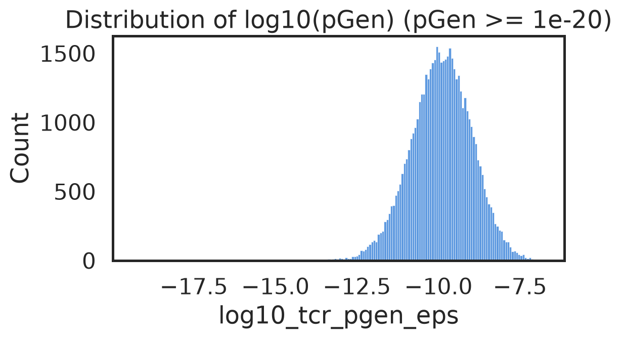
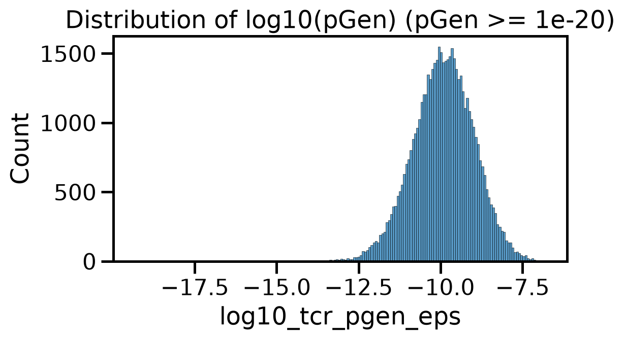
Two TCRs have dramatically lower pGen than the rest. Let’s take those out, just for plotting:

Code

n_verylow_pgens = sum(pdf_cmv_ecocluster_2026.tcr_pgen < 1e-20)
print(f"TCRs with very low pGen (< 1e-20): {n_verylow_pgens}")
pdf_notlow_pgen = pdf_cmv_ecocluster_2026[pdf_cmv_ecocluster_2026.tcr_pgen >= 1e-20]
print(f"Plotting on TCRs with pGen >= 1e-20: {len(pdf_notlow_pgen)} of {len(pdf_cmv_ecocluster_2026)} TCRs")

TCRs with very low pGen (< 1e-20): 2
Plotting on TCRs with pGen >= 1e-20: 52445 of 52447 TCRs

5.5.1 Look at the distribution of pGen, full ECOcluster.

Code

f, ax = plt.subplots()
sns.histplot(pdf_notlow_pgen.log10_tcr_pgen_eps, stat="count", ax=ax)
f.set_size_inches(6, 3)
ax.set_title("Distribution of log10(pGen) (pGen >= 1e-20)")
pdf_cmv_ecocluster_2026.tcr_pgen.describe()

count    5.244700e+04
mean     9.605719e-10
std      4.195277e-09
min      0.000000e+00
25%      2.970808e-11
50%      1.259289e-10
75%      5.217633e-10
max      1.710280e-07
Name: tcr_pgen, dtype: float64

That’s more meaningful when placed in context. As described in the manuscript, it’s notably narrower, with a higher median, then randomly selected TCRs from a large number of repertoires.

5.5.2 Does it differ by HLA class? Plot and test.

Code

f, ax = plt.subplots()
sns.boxplot(x="hla_class", y="log10_tcr_pgen_eps", data=pdf_notlow_pgen, ax=ax)
ax.set_title("Distribution of log10(pGen)\nby HLA class (pGen >= 1e-20)")
f.set_size_inches(4, 3)

mwu_p = mannwhitneyu(pdf_cmv_ecocluster_2026[pdf_cmv_ecocluster_2026.hla_class == "ci"].tcr_pgen,
              pdf_cmv_ecocluster_2026[pdf_cmv_ecocluster_2026.hla_class == "cii"].tcr_pgen,
              alternative="two-sided").pvalue
class_ii_is_higher = pdf_cmv_ecocluster_2026[pdf_cmv_ecocluster_2026.hla_class == "cii"].tcr_pgen.mean() > pdf_cmv_ecocluster_2026[pdf_cmv_ecocluster_2026.hla_class == "ci"].tcr_pgen.mean()
higher_class = "Class II" if class_ii_is_higher else "Class I"
print(f"2-sided Mann-Whitney U test p-value: {mwu_p:.3e}. Mean pGen is higher for {higher_class}.")

2-sided Mann-Whitney U test p-value: 1.220e-03. Mean pGen is higher for Class I.

The means aren’t very different, but Class I mean is significantly higher. That could be a consequence of the greater statistical power to associated TCRs with Class II alleles: In Class II, we can associate TCRs with lower pGen, that occur in a lower proportion of people with the allele.